Physical Qubits

2.1 Energy Levels

The eigenvalues of a Hamiltonian are energies. What do its eigenvectors do in time, and why can a third one spoil a qubit made of two? Finding the states that evolve only by a phase gives energy levels and transition frequencies. Projecting onto two of those levels then isolates exactly the term that a two-level model ignores.

2.1.1 Stationary states and frequencies

Which states does a Hamiltonian leave unchanged, apart from a phase? The evolution law answers this directly. If \(H\ket j=E_j\ket j\), then \(e^{-iHt/\hbar}\ket j=e^{-iE_jt/\hbar}\ket j\). The state only gains a phase, so every measurement probability stays fixed. Such an eigenvector is called a stationary state, and its eigenvalue \(E_j\) an energy level. A device with levels \(E_0\), \(E_1\), \(E_2\) is a device whose Hamiltonian has these eigenvalues.

Why does an energy difference set an oscillation frequency? Expand a general state in stationary states, \(\ket\psi=\sum_jc_j\ket j\), and write \(\dot c_j\) for the rate of change of an amplitude. The evolution law becomes \(i\hbar\dot c_j=E_jc_j\) for each level separately. A function whose derivative is proportional to itself is an exponential, so \(c_j(t)=c_j(0)e^{-iE_jt/\hbar}\). In a superposition of \(\ket0\) and \(\ket1\), the ratio \(c_1/c_0\) therefore gains the phase \(e^{-i(E_1-E_0)t/\hbar}\).

So \(\omega_{01}=(E_1-E_0)/\hbar\) is an angular frequency, in radians per second, while \(f_{01}=(E_1-E_0)/h\) counts cycles per second. Adding the same energy to every level multiplies the whole state by a common phase and changes no probability, so only energy differences matter. A 5 GHz splitting completes one cycle of relative phase every 0.2 ns. The frequency describes a turning phase, not a particle jumping back and forth between levels.

2.1.2 The two-level approximation

Now suppose the device has a third level, and we want to use only the lowest two. Can we simply ignore the third? Let \(P=\ket0\bra0+\ket1\bra1\) project onto the chosen pair, and \(Q=I-P\) onto the rest. Apply \(P\) to the evolution law and insert \(I=P+Q\) in front of the state:

\[i\hbar\,\frac{d(P\ket\psi)}{dt}=PHP\ket\psi+PHQ\ket\psi.\]

The first term is the qubit model. The second couples the qubit to the omitted level. Calling two levels a qubit does not make that term zero.

When is the second term harmless? If \(H\) is the free Hamiltonian, diagonal in the energy basis, then \(PHQ=0\) and the pair evolves on its own exactly. Trouble starts when a control adds terms that connect levels. A control tuned to the 0–1 frequency then also acts on any other transition that has the same frequency.

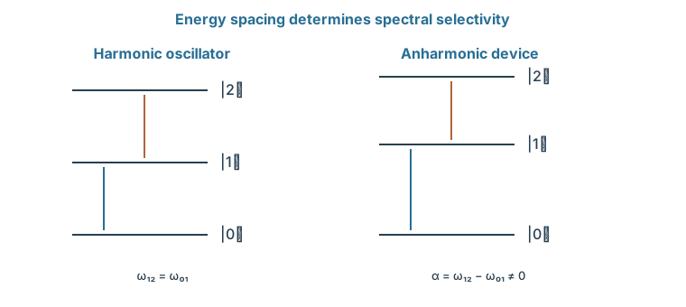
This is where the spacing of the levels matters. For equally spaced levels \(\omega_{12}=\omega_{01}\), so frequency alone cannot address the 0–1 transition without the 1–2 transition. We measure the departure from equal spacing by the anharmonicity \(\alpha=\omega_{12}-\omega_{01}\). A large \(|\alpha|\) is what lets a control at \(\omega_{01}\) leave the 1–2 transition nearly untouched. How large it must be depends on the strength and duration of the control.

2.2 Qubit Encodings

Two chosen levels are a starting point, but population can still escape them. How should escaped population be counted, and what decides whether a coupling can move it at all? Defining the computational subspace fixes the bookkeeping for leakage. Asking which matrix entries a control has, and how far a mismatched coupling can move population, then bounds the escape.

2.2.1 Computational subspaces

What exactly is the qubit inside a larger system? It is the two-dimensional subspace spanned by the encoded states, called the computational subspace. The encoded states need not be energy levels. They can be two paths of one photon, or joint states of several particles. Once chosen, the encoding fixes what a physical operator means logically. For a photon in two paths, an energy shift on one path acts as a relative phase, while losing the photon removes it from the entire subspace.

How should we report leakage? Suppose a measurement resolves all three levels of a device and reports \(p_0,p_1,p_2\), summing to one. The leakage is \(L=p_2\). A procedure that discards level-2 outcomes reports \(p_1/(1-L)\) instead. With \((p_0,p_1,p_2)=(0.45,0.45,0.10)\), the retained sample looks exactly balanced, although a tenth of the population leaked. Reporting both the unconditional probabilities and the retained fraction removes that ambiguity.

2.2.2 Leakage and selection rules

Which levels can a control connect? A control adds an operator \(D\) to the Hamiltonian with some strength. In the energy basis, the entry \(\bra mD\ket n\) couples the amplitudes of levels \(n\) and \(m\). If that entry vanishes, the control cannot move population directly from \(n\) to \(m\). A vanishing entry of this kind is a selection rule. It usually comes from a symmetry of the system, so a different field or a broken symmetry can restore the coupling. A selection rule therefore names both the operator and the symmetry.

When the entry does not vanish, how much population can it move? Take the simplest case. Two levels have energies that differ by \(\hbar\Delta\), and a constant coupling of strength \(\hbar\Omega/2\) joins them. Dropping the common energy,

\[H/\hbar=\tfrac12(-\Delta Z+\Omega X).\]

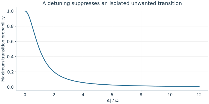
Squaring gives \(H^2/\hbar^2=(\Delta^2+\Omega^2)I/4\), because \(Z^2=X^2=I\) and \(XZ+ZX=0\). Write \(\Omega_R=\sqrt{\Omega^2+\Delta^2}\) and \(N=(-\Delta Z+\Omega X)/\Omega_R\), so that \(H/\hbar=\Omega_RN/2\) with \(N^2=I\). The even and odd split of the exponential gives \(e^{-iHt/\hbar}=\cos(\Omega_Rt/2)I-i\sin(\Omega_Rt/2)N\). Since \(\bra1N\ket0=\Omega/\Omega_R\), the probability of moving from 0 to 1 is

\[P_{0\to1}(t)=\frac{\Omega^2}{\Omega_R^2}\sin^2\frac{\Omega_Rt}{2}\le\frac{\Omega^2}{\Omega^2+\Delta^2}.\]

An energy mismatch caps the transfer, however long we wait. At \(|\Delta|=10\Omega\) the cap is \(1/101\). This is the mechanism that anharmonicity relies on: the unwanted transition sees a large mismatch. A drive, viewed in suitable coordinates, will turn out to give exactly this matrix, with \(\Delta\) the mismatch between drive and transition frequencies. The bound covers one isolated transition under a constant coupling. Several unwanted levels, pulse edges, or repeated gates can each break it.

2.3 Effective Dynamics

Our two-level formulas are exact for constant Hamiltonians. Yet free evolution alone turns the relative phase billions of times a second, and that known fast motion can hide the slow changes a control makes. How do we remove it, and how do we know a reduced model is right? Factoring out a reference evolution gives the rotating frame and the detuning. Asking which predictions a calibrated model has not yet seen then gives a test of the whole approximation.

2.3.1 Hamiltonians and rotating frames

What is the qubit Hamiltonian in Pauli form? With \(Z=\ket0\bra0-\ket1\bra1\), the energies \(0\) and \(\hbar\omega_{01}\) give \(H_0=\hbar\omega_{01}(I-Z)/2\). Dropping the common energy \(\hbar\omega_{01}/2\) leaves \(H_0=-\hbar\omega_{01}Z/2\). The minus sign comes from labelling level 1 as the higher-energy state.

Under \(H_0\) alone, the relative phase turns at \(\omega_{01}\). We know this motion exactly. Can we remove it and follow only the slow changes that a weak control adds? Suppose we describe the state relative to a chosen reference evolution \(R(t)=e^{-iH_{\rm ref}t/\hbar}\), writing \(\ket\psi=R(t)\ket{\psi_r}\). The evolution law gives \(i\hbar\dot R\ket{\psi_r}+i\hbar R\,d\ket{\psi_r}/dt=HR\ket{\psi_r}\). Multiplying by \(R^\dagger\) shows that \(\ket{\psi_r}\) evolves under

\[H_r=R^\dagger HR-i\hbar R^\dagger\dot R.\]

Choose the reference \(H_{\rm ref}=-\hbar\omega_dZ/2\), a phase turning at some chosen angular frequency \(\omega_d\). This \(R\) commutes with \(H_0\), and \(-i\hbar R^\dagger\dot R=-H_{\rm ref}\). So the free part becomes

\[H_r=-\hbar(\omega_{01}-\omega_d)Z/2.\]

In these coordinates the phase turns only at the difference \(\Delta=\omega_{01}-\omega_d\), called the detuning. If \(\omega_d=\omega_{01}\), the free evolution disappears altogether. Such coordinates are called a rotating frame. The frame is a choice of description, whereas changing the frequency of a physical field is an experimental action. Keeping the two apart prevents a calculation from producing a gate that no field supplied.

2.3.2 Testing the approximation

A reduced model fits the data it was calibrated on. How do we test it on data it has not seen? We estimate a transition frequency with weak spectroscopy and calibrate a rotation at one amplitude. Then we predict the response at another amplitude and detuning. An amplitude-dependent frequency shift, or an extra oscillation, shows that the model has omitted a level or a correction to the drive.

Errors also accumulate from pulse to pulse. Suppose one pulse leaves an unwanted amplitude \(\epsilon\), with population \(|\epsilon|^2\). If successive pulses add that amplitude with the same phase, after \(N\) pulses the amplitude is about \(N\epsilon\) and the population about \(N^2|\epsilon|^2\), while this stays small. Amplitudes add before they are squared. If the phases are instead random, the populations add on average, giving about \(N|\epsilon|^2\). So a small one-pulse leakage does not predict a long circuit until we know how the phases of successive errors are related.

Within the chosen subspace, how does an oscillating field produce a rotation, and why must its frequency match the transition?

Models and further derivations: Krantz et al.: Hamiltonians, levels, and control models. Numerical examples in this chapter are illustrative, not device specifications.