Superconducting Circuits

8.1 Circuit Qubits

A capacitor and an inductor exchange electric and magnetic energy, like a mass on a spring. Why can we not simply call their two lowest levels a qubit, and what element changes that? Quantizing the circuit gives an equally spaced ladder. A Josephson junction adds a nonlinear energy, and in the transmon regime that energy makes the ladder slightly unequal.

8.1.1 Oscillators and Josephson junctions

What does a capacitor connected to an inductor do? Let \(C\) be the capacitance and \(L\) the inductance. Let \(Q\) be the capacitor's charge and \(\Phi\) the flux, the time integral of the voltage across the inductor. Their stored energy is \(H=Q^2/(2C)+\Phi^2/(2L)\). The circuit equations \(\dot\Phi=Q/C\) and \(\dot Q=-\Phi/L\) give \(\ddot\Phi=-\Phi/(LC)\): an oscillator with angular frequency \(\omega=1/\sqrt{LC}\).

What are its quantum levels? We take one physical input: in the quantum description, \(\Phi\) and \(Q\) become Hermitian operators with \([\Phi,Q]=i\hbar\), the same rule that holds for a particle's position and momentum. Now define \(a\) through

\[\Phi=\Phi_{\rm zpf}(a+a^\dagger),\qquad Q=-iQ_{\rm zpf}(a-a^\dagger),\qquad[a,a^\dagger]=1.\]

Then \([\Phi,Q]=2i\Phi_{\rm zpf}Q_{\rm zpf}\), so the rule holds if \(\Phi_{\rm zpf}Q_{\rm zpf}=\hbar/2\). Choosing \(\Phi_{\rm zpf}=\sqrt{\hbar Z_c/2}\) and \(Q_{\rm zpf}=\sqrt{\hbar/(2Z_c)}\), with impedance \(Z_c=\sqrt{L/C}\), satisfies it. With this choice \(Q_{\rm zpf}^2/C=\Phi_{\rm zpf}^2/L=\hbar\omega/2\). Substituting into the energy, the terms with \(a^2\) and \((a^\dagger)^2\) cancel, and what remains is \(H=\hbar\omega(a^\dagger a+\tfrac12)\).

Why are the eigenvalues of \(a^\dagger a\) whole numbers? From \([a,a^\dagger]=1\) we get \([a^\dagger a,a]=-a\). So if \(a^\dagger a\ket\nu=\nu\ket\nu\), then \(a\ket\nu\) is an eigenvector with eigenvalue \(\nu-1\): \(a\) steps down by one. Its squared length is \(\bra\nu a^\dagger a\ket\nu=\nu\), which cannot be negative. Stepping down repeatedly would eventually produce a negative eigenvalue, unless the ladder ends at a state with \(a\ket0=0\). So \(\nu=0,1,2,\ldots\), and the energies are \(E_n=\hbar\omega(n+\tfrac12)\). The squared length also gives \(a\ket n=\sqrt n\ket{n-1}\). This is the lowering operator we used for an oscillating mediator, now derived for a circuit.

Equal spacing is exactly what prevents a resonant drive from singling out the lowest pair. Some element must make the energy nonlinear. That element needs a physical input of its own. In certain metals cooled to very low temperature, electrons bind into pairs that flow without resistance. This state is called superconductivity, and each pair carries charge \(2e\). A Josephson junction is a thin insulating barrier between two superconductors, through which pairs can tunnel.

Physical input (Josephson energy). The junction stores energy \(-E_J\cos\varphi\), where \(\varphi=2\pi\Phi/\Phi_0\) and \(\Phi_0=h/(2e)\) is the flux quantum.

Replacing the inductor's quadratic energy by this cosine makes successive transition frequencies differ, and that makes selective qubit control possible. The device must be cold for two reasons: superconductivity requires it, and the thermal excited population must be small.

8.1.2 The transmon regime

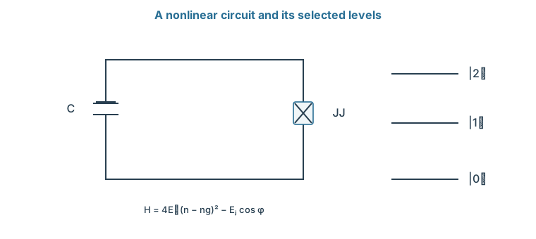
How unequal does the junction make the ladder? Count the charge in units of pairs: \(Q=2e(n-n_g)\), where \(n\) is the number of pairs that have tunnelled and \(n_g\) is an offset charge set by a gate voltage and by stray charges nearby. The charging energy becomes \(4E_C(n-n_g)^2\), with \(E_C=e^2/(2C)\). Together with the junction,

\[H=4E_C(n-n_g)^2-E_J\cos\varphi.\]

When \(E_J/E_C\) is large, \(\varphi\) stays near the bottom of the cosine, so we expand:

\[-E_J\cos\varphi\simeq-E_J+\tfrac12E_J\varphi^2-\tfrac1{24}E_J\varphi^4.\]

The quadratic part is an LC oscillator in disguise. Because \(\varphi=2e\Phi/\hbar\), the quantization rule becomes \([\varphi,n]=i\). Matching \(4E_Cn^2+E_J\varphi^2/2\) to the LC energy gives the level spacing \(\sqrt{8E_JE_C}\), and \(\varphi=\varphi_{\rm zpf}(a+a^\dagger)\) with \(\varphi_{\rm zpf}^2=\sqrt{2E_C/E_J}\).

What does the quartic term do to the levels? We quote the standard first-order result of perturbation theory. When a small term is added to a Hamiltonian with known levels, each level shifts, to first order, by the expectation value of that term in the unperturbed state. Here \(\bra n(a+a^\dagger)^4\ket n=6n^2+6n+3\), so level \(n\) shifts by \(-E_C(6n^2+6n+3)/12\). Subtracting neighbouring energies gives

\[\hbar\omega_{01}\simeq\sqrt{8E_JE_C}-E_C,\qquad\hbar(\omega_{12}-\omega_{01})\simeq-E_C.\]

The anharmonicity is about \(-E_C\). This device, a junction with a large shunting capacitance so that \(E_J\gg E_C\), is called a transmon. The formulas are a weak-anharmonicity approximation, not an exact spectrum. They also miss a second benefit of the large ratio. The levels depend on the stray offset \(n_g\), a dependence called charge dispersion. The full periodic model shows, as a quoted result, that this dependence falls exponentially with \(\sqrt{8E_J/E_C}\), so the transmon is nearly insensitive to stray charge.

8.2 Control and Coupling

With a transmon's levels known, how do we drive one, and how do two of them interact? A voltage on a nearby electrode gives the familiar resonant drive, with leakage set by the small anharmonicity. Capacitive coupling between circuits gives exchange, and tuning levels close to one another gives a conditional phase.

8.2.1 Microwave gates

How does a voltage rotate a transmon? A drive electrode adds a time-dependent voltage, and therefore a term that couples to the charge \(n\). Projecting its matrix elements onto the lowest two levels gives the resonant drive term \(\hbar\Omega\cos(\omega_dt-\phi)X\), and all of single-qubit control follows. The next level is still present, though. Its detuning from the drive is about the anharmonicity, which is far smaller than the transition frequency.

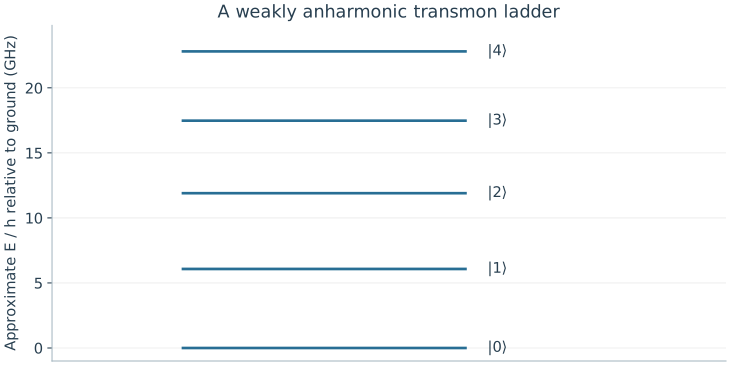
For the illustrative values \(E_C/h=0.25\) GHz and \(E_J/h=20\) GHz, \(f_{01}\simeq6.075\) GHz and \(f_{12}\simeq5.825\) GHz. By the pulse-spectrum argument, a pulse much longer than \(1/(2\pi\times0.25\,\text{GHz})\), about 0.6 ns, and much weaker than the anharmonicity distinguishes them. A stronger, shorter pulse can excite both. Initialization uses thermal relaxation or measurement-based reset. The residual excited and leaked populations must be measured, since the refrigerator temperature alone does not fix them.

8.2.2 Resonators and entangling gates

How do two circuits interact? A capacitor between them adds an energy proportional to the product of their charges. In the oscillator description each charge is proportional to \(i(a^\dagger-a)\), so the product contains \(a^\dagger b\), \(ab^\dagger\), \(ab\), and \(a^\dagger b^\dagger\), where \(b\) lowers the second circuit. Near resonance, in the rotating frame, the last two turn at the sum of the two frequencies, and the rotating-wave argument drops them. What remains is excitation exchange, \(\hbar g(a^\dagger b+ab^\dagger)\). Keeping two levels per circuit replaces \(a\) by \(\ket0\bra1\), and the coupling becomes \(\hbar g(XX+YY)/2\), the exchange interaction whose swap dynamics we already know.

Can a transmon pair also produce a conditional phase? Suppose only \(\ket{11}\) gains an extra energy \(\delta E\) for a time \(t\). Its amplitude gains \(e^{-i\delta Et/\hbar}\), and choosing that phase to be π gives a controlled sign after local phase corrections. One way to produce such a shift uses the third level. When two coupled levels are tuned toward each other, they repel instead of crossing, which is called an avoided crossing. Tuning \(\ket{11}\) close to the non-computational state \(\ket{02}\) pushes the energy of \(\ket{11}\) alone. Such a gate passes through the third level, so it must be analysed in the larger space to predict leakage, and it must end back in the qubit basis.

8.3 Readout and Scaling

A processor must also read its qubits, and it must keep working as it grows. How does a microwave signal learn the qubit's state, and what limits a large array? Coupling the qubit to a detuned resonator shifts the resonator's frequency by an amount that depends on the qubit's state. Residual couplings, wiring, and heat then set the cost of adding qubits.

8.3.1 Dispersive measurement

How can a qubit change a signal without being driven between its levels? Couple it to a resonator whose frequency \(\omega_r\) is far from the qubit frequency \(\omega_q\). With one excitation shared between them, the Hamiltonian is a two-by-two matrix with diagonal \(\hbar\omega_q,\hbar\omega_r\) and off-diagonal \(\hbar g\). Its eigenvalues are

\[\hbar\frac{\omega_q+\omega_r}2\pm\hbar\sqrt{\frac{\Delta^2}4+g^2},\qquad\Delta=\omega_q-\omega_r.\]

For \(|g/\Delta|\ll1\), expanding the square root shifts the two uncoupled levels by about \(\pm\hbar g^2/\Delta\).

What does this do to the resonator? We quote the result of the same calculation over the whole qubit–resonator ladder, for a two-level qubit. The resonator frequency shifts by \(+\chi\) or \(-\chi\), depending on the qubit's state, with \(\chi=g^2/\Delta\). This weak-coupling, far-detuned regime is called dispersive. A probe tone near the resonator frequency therefore leaves with a phase that depends on the qubit's state, and that phase is the readout signal. A transmon's extra levels change the value of \(\chi\), and a strong probe can break the expansion. So the readout is calibrated at the actual probe power and acquisition window.

8.3.2 Materials, wiring, and crosstalk

What changes when many circuits share a chip? A small residual frequency error \(\delta\omega\) accumulates phase \(\delta\omega t\). A residual ZZ coupling between neighbours accumulates a conditional phase even during gates meant to be independent. These errors depend on time, on layout, and on which operations run together, so isolated gate measurements cannot fully predict an array.

Each added qubit also brings control lines, readout resonators, possible frequency collisions with its neighbours, and heat at the cold stages. A hypothetical installation of 1000 lines, each delivering 10 nW, already loads its stage with 10 μW before any active dissipation. This is an accounting example, not a refrigerator specification. A fabricated layout becomes a processor only when its controls can operate its usable qubits in parallel within such budgets.

An atom offers levels that nature makes identical from one atom to the next, but two atoms held apart in a trap do not touch. What can supply the coupling between them?

Models and further derivations: Koch et al.: transmon spectrum and design; Blais et al.: circuit quantum electrodynamics. Numerical examples in this chapter are illustrative, not device specifications.