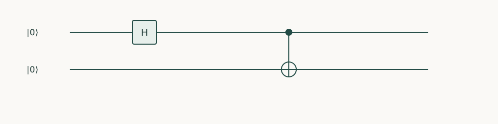
Starting point: Earlier programming chapters; relevant constructions from Quantum Computing and Quantum Algorithms.
Anchor example: Prepare a Bell pair and predict its measured bit strings.
This lesson includes explanations, worked examples, and problems with solutions. Advanced results whose proofs are outside the chapter are identified explicitly.
Our coin program had one qubit and one classical bit, so every outcome was a single character and nothing could be misread. With two qubits, a program has to say which wire a gate acts on, which classical bit receives which measurement, and which character of a string such as 01 belongs to which qubit. A circuit diagram leaves some of these choices to the reader’s eye.
How, then, does a circuit diagram become an unambiguous program? We work with the Bell pair, whose ideal outcomes are only 00 and 11. That symmetry is exactly the problem: a program that confuses qubit 0 with qubit 1 still gives the right counts. So we first fix how registers and gate order are written, then design an asymmetric experiment that exposes the ordering of bit strings, and finally learn to inspect a circuit and compare it with the evolution we predict.
By the end, every index in a two-qubit program will have one meaning.
3.1 Registers and Gates
The Bell pair comes from H on one qubit followed by a CNOT. To write it as a program we must name the qubits, name the bits that receive their measurements, and put the gates in order. Only equal bits should appear when we measure, but a symmetric result can hide an ordering mistake, so we will need an asymmetric test before trusting the program. We begin with the names.
3.1.1 Quantum and classical registers
What does QuantumCircuit(2) actually create? It creates two quantum wires, numbered 0 and 1. A group of qubits addressed together is called a quantum register. Qubits carry quantum states, but measurement results are ordinary bits, and they need somewhere to go. A classical register is a row of classical bits that receives measurement records.
Gates refer to qubits by number. In bell.h(0) followed by bell.cx(0, 1), the first argument of cx is the control and the second is the target. So qubit 0 gets the H and controls the CNOT, and qubit 1 is flipped when qubit 0 is 1.
That fixes what each instruction does. It does not yet fix how a two-qubit state or a measured string is written down. When we computed the Bell state by hand, we wrote qubit 0 as the first label. Whether Qiskit does the same is a question we will settle by experiment.
3.1.2 Gate order and circuit composition
Each method call appends its gate after the ones already there, so the program lists gates in the order they happen. How does that order appear in the matrix of the whole circuit?
Suppose we apply \(U\) and then \(V\). The state becomes \(V(U\ket\psi)=(VU)\ket\psi\). The gate applied last stands on the left. So a program that appends \(U_1,U_2,\dots,U_k\) has the matrix \(U_k\cdots U_2U_1\), the reverse of the reading order.
Programs also need to join circuits. The method compose places one circuit after another and returns the combined circuit. Its qubits argument says which wires of the larger circuit receive the smaller circuit’s wires. Writing qubits=[1, 0], for instance, sends the small circuit’s qubit 0 to wire 1. Without such a mapping, a component built for one wire order would be silently attached in another.
A composed circuit may also appear as one labelled box. A box can stand for many elementary gates, and its size on the page says nothing about that number. The method decompose() replaces each box by its contents, one level at a time, so we can see what it costs.
3.2 Measurement
The gates are now in order, but the result of a program is a string of classical bits. Two choices stand between a qubit and a character of that string: which bit stores the qubit’s measurement, and where that bit appears in the printed string. We make the first choice explicit, then use an asymmetric experiment to discover the second.
3.2.1 Mapping qubits to classical bits
Who decides which classical bit receives which qubit’s outcome? We do, or a default does. The coin program used measure_all(), which adds a register named meas and measures qubit \(j\) into bit \(j\). The method measure(qubit, clbit) instead names one qubit and one classical bit, so we can choose any mapping.
Suppose we measure qubit 0 into bit 1 and qubit 1 into bit 0. The quantum state is unchanged, yet every result string now describes the qubits in the swapped order. A count string describes classical storage, not wires. So decoding a result requires knowing the measurement mapping.
3.2.2 Bit strings and tensor-product ordering
With the default mapping, which character of a printed string belongs to qubit 0? The Bell pair cannot tell us, because 00 and 11 read the same in both directions. So we need a state that is not symmetric. Suppose we apply X to qubit 0 alone. Then qubit 0 is 1 and qubit 1 is 0. If Qiskit wrote qubit 0 first, as we did by hand, we would see 10.
The companion asks for the probabilities of this state, and the answer is {"01": 1.0}. So qubit 0 is the rightmost character. Qiskit reads a bit string as a binary number, with qubit 0 as the least significant digit, just as the ones digit of an ordinary number sits on the right. A two-qubit basis state is written \(\ket{q_1q_0}\), and its position in the state vector is \(k=q_0+2q_1\). Our state is \(\ket{01}\), at index 1.
The tensor product follows the same convention. The state vector is \(\ket{q_1}\otimes\ket{q_0}\), so a gate \(A\) on qubit 0 alone has the matrix \(I\otimes A\), with \(A\) on the right. The Bell state \((\ket{00}+\ket{11})/\sqrt2\) is the same in both conventions, which is why the Bell test could not catch a mistake. A drawing with qubit 0 at the top does not change any of this. It is a picture, not a reordering of the mathematics.
Problem 3.1. What state results from X on qubit one alone?
Worked solution
It is |10〉, with state-vector index two. This is the opposite single-bit position from X on qubit zero.
3.3 Circuit Inspection
We now know what every index means. Can we confirm that the program we wrote is the circuit we meant? Two kinds of evidence are available: what the circuit looks like, and what it computes. We take the picture first, then compare the computed results with our prediction.
3.3.1 Drawing and decomposing circuits
The quickest check is to look. draw(output="text") prints a drawing made of characters, so it needs no plotting software. We read its wires from left to right in time, and qubit 0 is the top wire. The returned bit strings still follow the classical register order, with qubit 0 on the right. So the top-to-bottom order of the drawing is the right-to-left order of a result string.
A drawing can mislead in one way. A familiar-looking box may hide arithmetic or gates with many controls. When a box appears, decompose() shows what it contains, and count_ops() counts the gates of each kind. A compact picture is not a small circuit.
3.3.2 Comparing code with predicted evolution
What should the program’s numbers be? The Bell state is \((\ket{00}+\ket{11})/\sqrt2\), so ideal measurements give 00 and 11, each with probability one half, and never 01 or 10. The exact split between 00 and 11 fluctuates from run to run, so the test cannot demand it. What it can demand is that no other string ever appears.
The companion repeats the steps of the coin program on one line. Each dot applies to the result of everything to its left. The expression set(counts) makes a set, a collection without order or repeats, holding the keys of the dictionary. The test <= between sets asks whether the first is contained in the second. So the first check says that every observed string is 00 or 11. The second check is the asymmetric experiment, computed exactly with probabilities_dict().
"""Runnable companion for Quantum Programming, Chapter 3."""
from qiskit import QuantumCircuit
from qiskit.primitives import StatevectorSampler
from qiskit.quantum_info import Statevector

bell = QuantumCircuit(2)
bell.h(0)
bell.cx(0, 1)
bell.measure_all()
counts = StatevectorSampler(seed=8).run([bell], shots=1024).result()[0].data.meas.get_counts()
assert set(counts) <= {"00", "11"}
# An asymmetric check is essential: a Bell state hides reversed bit order.
asymmetric = QuantumCircuit(2)
asymmetric.x(0)
assert Statevector.from_instruction(asymmetric).probabilities_dict() == {"01": 1.0}
print(bell.draw(output="text"))
print(counts)
With seed 8, the run printed 533 counts of 00 and 491 of 11, and no other strings. Is that enough to show that the two qubits are entangled?
Not yet. Consider a device that prepares \(\ket{00}\) half the time and \(\ket{11}\) otherwise. Such a random choice between states is a classical mixture. It gives exactly the same measured counts. To tell the two apart, we apply H to both qubits before measuring. On the Bell state, H on both qubits gives \((\ket{{+}{+}}+\ket{{-}{-}})/\sqrt2\). Expanding, \(\ket{{+}{+}}=(\ket{00}+\ket{01}+\ket{10}+\ket{11})/2\) and \(\ket{{-}{-}}=(\ket{00}-\ket{01}-\ket{10}+\ket{11})/2\), so the 01 and 10 terms cancel and the Bell state returns. We still see only 00 and 11. But H on both sends \(\ket{00}\) to \(\ket{{+}{+}}\) and \(\ket{11}\) to \(\ket{{-}{-}}\), and each of these gives all four strings with probability one quarter. Testing in this second basis exposes the difference.
Problem 3.2. Would counts containing only 00 and 11 prove entanglement?
Worked solution
No. A classical mixture of \(\ket{00}\) and \(\ket{11}\) has the same computational-basis distribution. Applying H to both qubits before measurement distinguishes them: the Bell state still gives only 00 and 11, while the mixture gives all four strings equally often.
Problem 3.3. Why include a text drawing in a runnable example?
Worked solution
It makes the appended gate order and wire targets inspectable. The numerical test still supplies the stronger check of the circuit’s action.
Bell-pair preparation. A Hadamard followed by CNOT makes (|00⟩+|11⟩)/√2. The first wire is the control.
Sampled counts gave us only indirect evidence about the state. Since a simulator computes the full state anyway, could we compare a circuit with its vector and its matrix directly?
Quantum and classical registers give structured names to wires, while multi-qubit gates such as cx, cz, and ccx require explicit control-to-target ordering.
Barriers prevent compiler passes from merging or reordering gates across diagnostic boundaries without altering the circuit’s unitary matrix.
Inspecting circuit depth, gate counts, and nonlocal two-qubit layers early catches scalability bottlenecks before transpilation.
Questions and worked problems
These exercises draw on the whole chapter. Attempt each question before opening a hint, explain your reasoning, then compare it with the worked solution.
A three-qubit circuit applies X only to qubit 2. Predict its bit-string label and its statevector index before running it.
Hint 1
Qubit 0 is the rightmost (least significant) bit.
Hint 2
Label \(q_2q_1q_0\).
Worked solution
The label is 100 and the index is \(4\): qubit 2 is the most significant of three bits. probabilities_dict returns {'100': 1.0}. Reading labels left to right as qubits 0, 1, 2 would wrongly predict 001.
Qubit 0 is flipped to 1, and qubit 1 is left at 0. The circuit then measures qubit 0 into classical bit 1 and qubit 1 into classical bit 0. What bit string appears in the counts?
Hint 1
Count strings are written with classical bit 0 on the right.
Hint 2
Classical bit 1 holds qubit 0’s value.
Worked solution
Classical bit 1 receives \(1\) and classical bit 0 receives \(0\), and count strings list classical bits from highest to lowest, so every shot gives 10. The physical state is the same \(\ket{q_1q_0}=\ket{01}\) as without the swapped mapping; only the storage changed. Decoding counts requires knowing the measurement map.
For the state prepared by X on qubit 0 of two qubits, predict the expectation values of the Pauli labels ZI and IZ.
Hint 1
The rightmost character acts on qubit 0.
Hint 2
\(\langle Z\rangle=+1\) on \(\ket0\) and \(-1\) on \(\ket1\).
Worked solution
ZI acts with \(Z\) on qubit 1, which is \(\ket0\): expectation \(+1\). IZ acts on qubit 0, which is \(\ket1\): expectation \(-1\). Swapping the two predictions is the typical symptom of reading Pauli labels in the wrong order.
import numpy as np
from qiskit.quantum_info import Statevector, SparsePauliOp

state = Statevector.from_label("01")
assert np.isclose(state.expectation_value(SparsePauliOp("ZI")), 1)
assert np.isclose(state.expectation_value(SparsePauliOp("IZ")), -1)
A Bell-pair subcircuit (H on its qubit 0, CX from 0 to 1) should be placed on qubits 2 and 0 of a three-qubit circuit. A student writes the code below and finds that big has no instructions. (a) Why? (b) Fix it. (c) Predict the resulting state’s labels.
from qiskit import QuantumCircuit

sub = QuantumCircuit(2)
sub.h(0)
sub.cx(0, 1)
big = QuantumCircuit(3)
big.compose(sub, qubits=[2, 0])
print(big.size())
Hint 1
compose returns a new circuit unless told otherwise.
Hint 2
qubits=[2, 0] maps subcircuit qubit 0 to qubit 2 and qubit 1 to qubit 0.
Worked solution
(a) compose returns a new circuit and leaves big unchanged unless inplace=True is given; the returned circuit was discarded. (b) Assign the result (or pass inplace=True). (c) The mapping puts H on qubit 2 and a CX from qubit 2 to qubit 0, entangling those two while qubit 1 stays \(\ket0\): the labels are 000 and 101, each with probability \(\frac12\).
from qiskit import QuantumCircuit
from qiskit.quantum_info import Statevector

sub = QuantumCircuit(2)
sub.h(0)
sub.cx(0, 1)
big = QuantumCircuit(3).compose(sub, qubits=[2, 0])
probabilities = Statevector.from_instruction(big).probabilities_dict()
assert abs(probabilities["000"] - 0.5) < 1e-12 and abs(probabilities["101"] - 0.5) < 1e-12
A Toffoli gate is drawn as one box. Decompose it once and count the resulting instructions. What does the count suggest about judging circuit cost from a drawing?
Hint 1
Use circuit.decompose() and count_ops().
Hint 2
Count the CNOTs and the \(T\)-type gates.
Worked solution
One level of decomposition gives \(6\) CNOTs, \(4\) \(T\) gates, \(3\) \(T^\dagger\) gates, and \(2\) Hadamards: fifteen elementary instructions for one drawn box. On fault-tolerant hardware the seven \(T\)-type gates dominate the cost. A compact drawing says nothing about resources; counts must be taken after decomposition, ideally after transpiling to the target gate set.
Counts of only 00 and 11 do not distinguish a Bell state from a classical mixture of \(\ket{00}\) and \(\ket{11}\). Write a check that does: apply H to both qubits before measuring, and compute the exact outcome probabilities for both preparations, using DensityMatrix for the mixture.
Hint 1
For the Bell state, \((H\otimes H)\ket{\Phi^+}=\ket{\Phi^+}\).
Hint 2
DensityMatrix.evolve applies a circuit to a mixed state.
Worked solution
After \(H\otimes H\), the Bell state still gives only 00 and 11, each with probability \(\frac12\), while the mixture gives all four outcomes with probability \(\frac14\). Exact probabilities make the test deterministic; in an experiment, the same comparison is made with sampled counts and a tolerance. Checking a second basis is what certifies coherence.
import numpy as np
from qiskit import QuantumCircuit
from qiskit.quantum_info import Statevector, DensityMatrix

bell = QuantumCircuit(2)
bell.h(0)
bell.cx(0, 1)
bell.h([0, 1])
bell_probs = Statevector.from_instruction(bell).probabilities_dict()
assert np.isclose(bell_probs["00"], 0.5) and np.isclose(bell_probs["11"], 0.5)

rotate = QuantumCircuit(2)
rotate.h([0, 1])
mixture = 0.5 * DensityMatrix.from_label("00") + 0.5 * DensityMatrix.from_label("11")
mix_probs = mixture.evolve(rotate).probabilities_dict()
assert all(np.isclose(mix_probs[label], 0.25) for label in ["00", "01", "10", "11"])
Prepare a five-qubit GHZ state \((\ket{00000}+\ket{11111})/\sqrt2\) in two ways: a chain of CNOTs \(0\to1\to2\to3\to4\), and a tree in which qubit 0 controls 1 and 2, then qubit 1 controls 3 while qubit 0 controls 4. Compare their depths and verify that the states agree.
Hint 1
Gates on disjoint qubits can share a layer.
Hint 2
Compare circuit.depth() and Statevector equivalence.
Worked solution
The chain has depth \(5\) (H plus four sequential CNOTs); the tree has depth \(4\), because the CNOTs \(0\to2\) and \(1\to3\) run in the same layer. Both prepare the same state. For \(n\) qubits a tree needs depth about \(1+\lceil\log_2n\rceil\), against \(n\) for a chain, so the same mathematical state can be much shallower, an important difference when qubits decohere while waiting.
from qiskit import QuantumCircuit
from qiskit.quantum_info import Statevector

chain = QuantumCircuit(5)
chain.h(0)
for k in range(4):
    chain.cx(k, k + 1)
tree = QuantumCircuit(5)
tree.h(0)
tree.cx(0, 1)
tree.cx(0, 2)
tree.cx(1, 3)
tree.cx(0, 4)
assert chain.depth() == 5 and tree.depth() == 4
assert Statevector.from_instruction(chain).equiv(Statevector.from_instruction(tree))
A student reads count strings from left to right in the same order as the wires in the text drawing, top to bottom, and concludes that 01 means “qubit 0 is 0 and qubit 1 is 1.” Show with a one-gate example that this is backwards.
Hint 1
The top wire in the drawing is qubit 0.
Hint 2
Apply X to qubit 0 and look at the label.
Worked solution
Apply X to qubit 0 only: the label is 01. The rightmost character is qubit 0, which is \(1\); the leftmost is qubit 1, which is \(0\). The drawing lists qubit 0 at the top, but the bit string lists it last, following the integer convention in which qubit 0 is the least significant bit. Every analysis that maps strings back to qubits must use this rule, or reverse the order explicitly.
from qiskit import QuantumCircuit
from qiskit.quantum_info import Statevector

circuit = QuantumCircuit(2)
circuit.x(0)
assert Statevector.from_instruction(circuit).probabilities_dict() == {"01": 1.0}
Some textbooks write the first qubit leftmost. Use Statevector.reverse_qargs() to convert the state of X on qubit 0 into that convention, and explain when such a conversion is appropriate and when it hides a bug.
Hint 1
reverse_qargs reverses the order of subsystems.
Hint 2
Convert once, at a clearly marked boundary.
Worked solution
In Qiskit’s convention the state is labelled 01; after reverse_qargs() it is labelled 10, matching a convention in which qubit 0 is written first. Converting is appropriate at a single, documented boundary, for example when comparing with a formula from a paper. Scattering conversions through a program, or reversing to make a failing test pass without understanding why, can mask a genuine wiring or measurement-map error.
from qiskit import QuantumCircuit
from qiskit.quantum_info import Statevector

circuit = QuantumCircuit(2)
circuit.x(0)
state = Statevector.from_instruction(circuit)
assert state.probabilities_dict() == {"01": 1.0}
assert state.reverse_qargs().probabilities_dict() == {"10": 1.0}
A circuit has two classical registers: a (one bit) measuring qubit 0, and b (two bits) measuring qubits 1 and 2. Qubit 1 is flipped. Predict the counts stored for each register and the combined string returned by join_data(). Why is it safer to read registers by name?
Hint 1
Each register is reported separately, with its own bit order.
Hint 2
In the joined string, the register added later appears on the left.
Worked solution
Register a reports 0 (qubit 0 is \(\ket0\)). Register b reports 01: its bit 0 holds qubit 1 (\(1\)) and its bit 1 holds qubit 2 (\(0\)). join_data() concatenates the registers, here as 010, with b on the left because it was added after a. Reading registers by name avoids depending on concatenation order, which changes if the circuit is built differently.
from qiskit import QuantumCircuit, QuantumRegister, ClassicalRegister
from qiskit.primitives import StatevectorSampler

q = QuantumRegister(3)
a = ClassicalRegister(1, "a")
b = ClassicalRegister(2, "b")
circuit = QuantumCircuit(q, a, b)
circuit.x(1)
circuit.measure(0, a[0])
circuit.measure([1, 2], b)
result = StatevectorSampler(seed=1).run([circuit], shots=5).result()[0]
assert result.data.a.get_counts() == {"0": 5}
assert result.data.b.get_counts() == {"01": 5}
assert result.join_data().get_counts() == {"010": 5}