Hybrid Quantum Programs

14.1 Parameterized Workflows

A variational program repeatedly prepares a state that depends on parameters and asks for its energy. If we started on a problem we could not solve, a wrong circuit and a weak optimizer would look the same. So we start with an energy we can compute by hand at every angle, and then decide how to request many evaluations of it.

14.1.1 Parameter binding and objectives

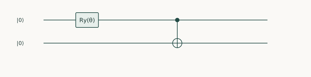
We apply \(R_y(\theta)\) to qubit 0 and then a CNOT from qubit 0 to qubit 1. This prepares \(\cos(\theta/2)\ket{00}+\sin(\theta/2)\ket{11}\). For the observable \(H=-ZZ-XX\), what energy \(E(\theta)=\langle H\rangle\) should the program report?

Write \(c=\cos(\theta/2)\) and \(s=\sin(\theta/2)\). Both \(\ket{00}\) and \(\ket{11}\) have equal bits, so \(\langle ZZ\rangle=c^2+s^2=1\). The operator \(XX\) exchanges \(\ket{00}\) and \(\ket{11}\), so \(\langle XX\rangle=2cs=\sin\theta\). Hence \[E(\theta)=-1-\sin\theta,\] with its minimum \(-2\) at \(\theta=\pi/2\), where the state is the Bell pair.

This curve is our oracle for testing the program: the computed energies must match it at every angle before we trust the loop on anything larger. The figure shows the circuit and the two measurements the energy needs, \(ZZ\) directly and \(XX\) after H on both wires.

14.1.2 Repeated estimation

An optimizer may ask for the energy at hundreds of angles. Should the program build a new circuit for each? No: as with parameter sweeps, we keep one symbolic circuit and pass the angles to the Estimator as an array of parameter rows. The companion does this for a grid of 101 angles. np.linspace(0, np.pi, 101) makes 101 equally spaced angles from 0 to \(\pi\). angles[:, None] turns that flat list into 101 rows of one value each. That is the general shape of a parameter array, one row per experiment and one column per circuit parameter, so the code states its workload explicitly rather than relying on Qiskit to interpret a flat list.

Each evaluation has a cost, even when the host loop is a single line. With the exact local Estimator there is no shot noise, which is right for this first debugging stage. On hardware, every energy would be an estimate, and the program would need to decide how many shots each term gets and how confident each value is.

14.2 Optimization Loops

A grid evaluates everywhere. An optimizer instead moves from one guess to a better one, so it needs a direction to move in, and a rule for when to stop. Both must be computed from estimates. We derive the direction first, then turn to stopping and to making runs comparable.

14.2.1 Gradients and classical updates

Which way should \(\theta\) move? The derivative \(E'(\theta)\) says, but the circuit gives us values of \(E\), not derivatives. Can we get the derivative exactly from a few values?

For our curve, try evaluating at \(\theta\pm\pi/2\): \[\frac{E(\theta+\pi/2)-E(\theta-\pi/2)}2=\frac{-\sin(\theta+\pi/2)+\sin(\theta-\pi/2)}2=-\cos\theta=E'(\theta).\] This is no accident. The rotation \(R_y(\theta)\) has entries \(\cos(\theta/2)\) and \(\pm\sin(\theta/2)\), and the energy is quadratic in them. Products such as \(\cos^2(\theta/2)\) and \(\cos(\theta/2)\sin(\theta/2)\) are combinations of \(1\), \(\cos\theta\) and \(\sin\theta\), so \(E(\theta)=A+B\cos\theta+C\sin\theta\) for some constants. The identity above holds for \(\cos\theta\) and \(\sin\theta\) separately, so it holds for every such \(E\). This is the parameter-shift rule: for a rotation generated by a single Pauli operator, the exact derivative is half the difference of two energies.

A gradient step then sets \(\theta\leftarrow\theta-\eta E'(\theta)\), where the step size \(\eta\) is called the learning rate. For one parameter, though, the grid is simpler and gives a reproducible baseline. Larger parameter spaces need more careful optimizers. No optimizer, however sophisticated, repairs a wrong circuit or a wrong objective.

14.2.2 Stopping criteria and reproducibility

When should the loop stop? “When the energy stops improving” sounds right, but with estimates the energy always fluctuates. An improvement smaller than its standard error is not evidence of progress. So a stopping rule combines a minimum improvement, judged against the uncertainty, with a fixed budget of evaluations.

Noise also distorts the direction. Estimated gradients can be biased, and in flat regions they are small compared with their errors, so the loop wanders. To compare two methods fairly, we fix their starting points and seeds. We also record failed runs and how results depend on the starting point. Choosing the best of many seeds afterwards understates both the classical and the quantum cost.

14.3 Applications

Our loop is a small instance of methods from the algorithms course. What do those methods promise, and what can a run like ours show about them? We treat the variational eigensolver first, since our example is one, then QAOA and the question of performance.

14.3.1 Variational eigensolvers

A variational eigensolver has three parts: a family of trial states, an estimator of the energy, and a classical search over parameters. Why should the lowest energy found say anything about the ground energy \(\lambda_{\min}\), the smallest eigenvalue of \(H\)? Expand a trial state in eigenvectors of \(H\), \(\ket\psi=\sum_kc_k\ket{e_k}\). Then \[\langle H\rangle=\sum_k|c_k|^2\lambda_k\ \ge\ \lambda_{\min}\sum_k|c_k|^2=\lambda_{\min}.\]

So every exact trial energy is an upper bound on the ground energy. This is the variational bound. It does not promise that the family contains the ground state, or that the search finds its best member. In our example the ground state of \(-ZZ-XX\) is the Bell pair, with energy \(-2\), and our family contains it at \(\theta=\pi/2\). An estimated energy can still fall below \(\lambda_{\min}\) through noise or bias. That breaks no law of quantum mechanics, but it does mean the estimate is wrong.

14.3.2 QAOA and performance comparisons

The quantum approximate optimization algorithm (QAOA), from the algorithms course, keeps the same loop and changes the trial family. Its states alternate evolutions under a cost observable, which encodes an optimization problem, and under a mixing observable. What would show that QAOA, or any variational method, is useful? A comparison with a good classical heuristic on the same instances, counting the evaluations spent on training as well as the final answer.

Our companion shows something much smaller: that the loop’s interface is correct. It compares every one of the 101 grid energies with \(-1-\sin\theta\), and then finds the minimum. np.argmin returns the position of the smallest entry, and int makes it an ordinary integer. The grid spacing is \(\pi/100\), so entry 50 is exactly \(\theta=\pi/2\), and the minimum is \(-2\). A solved two-qubit problem demonstrates correctness, not advantage.

"""Runnable companion for Quantum Programming, Chapter 14."""
import numpy as np
from qiskit import QuantumCircuit
from qiskit.circuit import Parameter
from qiskit.primitives import StatevectorEstimator
from qiskit.quantum_info import SparsePauliOp

theta = Parameter("theta")
qc = QuantumCircuit(2)
qc.ry(theta, 0); qc.cx(0, 1)
H = SparsePauliOp.from_list([("ZZ", -1), ("XX", -1)])
angles = np.linspace(0, np.pi, 101)
energies = StatevectorEstimator().run([(qc, H, angles[:, None])]).result()[0].data.evs
assert np.allclose(energies, -1 - np.sin(angles))
best = int(np.argmin(energies))
assert np.isclose(energies[best], -2)
print("Grid minimum:", angles[best], energies[best])

Companion script: chapter_14.py.

Our observables were sums of two Pauli strings. Advanced algorithms instead transform operators: they simulate time evolution, embed non-unitary matrices in unitaries, and apply polynomials to them. How do we implement such transformations with explicit resource costs?