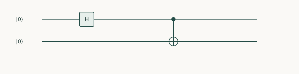
Starting point: Earlier programming chapters; relevant constructions from Quantum Computing and Quantum Algorithms.
Anchor example: Compare a small circuit with its matrix and state-vector predictions.
This lesson includes explanations, worked examples, and problems with solutions. Advanced results whose proofs are outside the chapter are identified explicitly.
So far we have judged circuits by their sampled counts, and we have seen how little counts can show. A Bell pair and a random choice between \(\ket{00}\) and \(\ket{11}\) give identical counts in the computational basis. Yet a simulator computes the complete state in order to produce those counts, so the information is there, inside the program.
How can simulation expose a program’s mathematical action? We start with the state a circuit produces. Asking what one qubit of a Bell pair is doing on its own shows that a state vector is not always enough, and the density matrix takes its place. A state describes only one input, so we then turn to the circuit’s full matrix, and to the observables whose averages experiments estimate. Finally we separate the numbers a simulator can print from those an experiment can recover.
Along the way we meet NumPy, the Python package for arrays of numbers.
4.1 State Representations
A simulator can show the state hidden inside a circuit, which makes it a debugging instrument: we can compare the program with its predicted action before sampling or noise enter. What form should that state take? A list of amplitudes is the natural first answer. We will find two situations it cannot describe, a random preparation and one part of an entangled pair, and one representation that handles both.
4.1.1 State vectors and density matrices
What exactly does Statevector.from_instruction(qc) compute? It starts every qubit in \(\ket0\), applies the circuit’s gates, and returns the \(2^n\) amplitudes in index order, with index \(k=q_0+2q_1+\cdots\). That works only for a circuit with no measurement or reset, since those are not unitary steps.
Now recall the device that prepares \(\ket{00}\) or \(\ket{11}\) with probability one half each. Can some single vector \(\psi\) describe it? To decide, we need a form in which predictions are easy to average. The average of an observable \(A\) in a pure state is \(\psi^\dagger A\psi\), and we can rewrite this using the trace, the sum of a matrix’s diagonal entries: \[\psi^\dagger A\psi=\sum_{j,k}\psi_j^*A_{jk}\psi_k=\operatorname{tr}\!\left(A\,\psi\psi^\dagger\right).\] A random preparation averages its predictions, so it gives \(\operatorname{tr}(A\rho)\) with \[\rho=\tfrac12\ketbra{00}{00}+\tfrac12\ketbra{11}{11}.\]
The matrix \(\rho\) is called a density matrix. For a mixture of states \(\psi_i\) with probabilities \(p_i\), it is \(\rho=\sum_ip_i\,\psi_i\psi_i^\dagger\), and every prediction is \(\operatorname{tr}(A\rho)\).
Is our \(\rho\) secretly of the form \(\psi\psi^\dagger\)? Any unit vector satisfies \((\psi\psi^\dagger)^2=\psi(\psi^\dagger\psi)\psi^\dagger=\psi\psi^\dagger\). Our \(\rho\) instead gives \(\rho^2=\tfrac14\ketbra{00}{00}+\tfrac14\ketbra{11}{11}=\rho/2\). So no vector describes the mixture, and we need the more general object. Qiskit’s DensityMatrix class holds it, and DensityMatrix(state) turns a vector into \(\psi\psi^\dagger\).
4.1.2 Composite systems and subsystem order
Density matrices settle a question vectors could not. In a Bell pair, what can we say about qubit 0 alone? Any test on qubit 0 alone uses an observable of the form \(I\otimes A\), with \(A\) on the right because qubit 0 is the right factor. For the Bell state \(\Phi=(\ket{00}+\ket{11})/\sqrt2\), \[\Phi^\dagger(I\otimes A)\Phi=\tfrac12\left(\bra0A\ket0+\bra1A\ket1\right)=\operatorname{tr}\!\left(A\,\tfrac I2\right).\] So every test on qubit 0 behaves as if that qubit had the density matrix \(I/2\). Since \((I/2)^2=I/4\), no vector describes it either.
The operation that produces a subsystem’s density matrix is the partial trace. To discard qubit 1, we sum over its label: \[(\rho_0)_{ab}=\sum_{c}\bra{c\,a}\rho\ket{c\,b},\] where the left label \(c\) belongs to qubit 1. For the Bell pair only \(c=a=b=0\) and \(c=a=b=1\) contribute, each giving \(\tfrac12\), so \(\rho_0=I/2\). In Qiskit, partial_trace(state, [1]) takes the list of subsystems to discard, not those to keep.
Is \(I/2\) just another way of writing \(\ket+\)? Both give zero and one with probability one half. But \[\ketbra++=\begin{pmatrix}\tfrac12&\tfrac12\\\tfrac12&\tfrac12\end{pmatrix},\qquad \frac I2=\begin{pmatrix}\tfrac12&0\\0&\tfrac12\end{pmatrix}.\] The average of X is \(\operatorname{tr}(X\rho)=\rho_{01}+\rho_{10}\), which is 1 for \(\ket+\) and 0 for \(I/2\). So an X-basis test tells them apart.
Problem 4.1. What does partial_trace(state,[1]) keep for two qubits?
Worked solution
It discards subsystem one and keeps subsystem zero. Confusing the two can pass unnoticed on symmetric states.
4.2 Operators and Observables
A state tells us what the circuit produced from one input, all zeros. A wrong circuit could still produce the right state from that input. And the averages we compared were computed from states one test at a time. We therefore need operators of two kinds: the circuit’s whole matrix, which covers every input, and the observables whose averages we predict.
4.2.1 Unitary operators
How can we check a circuit on every input at once? Its matrix does that, because column \(k\) of the matrix is the output for basis input \(k\). Operator(qc) builds this matrix for a circuit with no measurement or reset. For it to be a valid quantum evolution, it must be unitary, \(U^\dagger U=I\), and the companion checks this.
The check uses NumPy, imported as np. NumPy stores matrices as arrays and supplies matrix arithmetic. Operator(qc).data is the matrix as such an array. The method .conj() takes complex conjugates and .T transposes, so .conj().T is the dagger. The operator @ multiplies matrices, and np.eye(4) is the \(4\times4\) identity.
Why not test equality with ==? Computers store \(1/\sqrt2\) only approximately. In Python, (2**-0.5)**2 gives 0.5000000000000001, not 0.5, so an exact comparison can fail for a correct circuit. np.allclose instead accepts entries that agree within a small tolerance. Its default tolerance is far tighter than any mistake we are looking for, and far looser than these rounding errors.
How far does this check scale? An \(n\)-qubit unitary is a \(2^n\times2^n\) matrix, so it has \(2^n\cdot2^n=4^n\) complex entries. At 20 qubits that is about \(1.1\times10^{12}\) entries, roughly 18 terabytes at 16 bytes each. A full matrix is a check for small circuits only.
4.2.2 Pauli observables and expectation values
When we tested the Bell pair with H on both qubits, we inferred the result from counts. Can we predict such averages directly? The observables we need are Pauli strings: tensor products of \(I,X,Y,Z\), written as letters. Following the bit-order convention, the rightmost letter acts on qubit 0, so ZI means \(Z\) on qubit 1 and nothing on qubit 0.
Each Pauli string has eigenvalues \(\pm1\), so a single measurement of it gives \(+1\) or \(-1\), and its average lies between \(-1\) and \(1\). For the Bell state, the two Z outcomes always agree, so their product is always \(+1\) and \(\langle ZZ\rangle=1\). Since \(XX\) swaps \(\ket{00}\) with \(\ket{11}\), it leaves the Bell state unchanged, so \(\langle XX\rangle=1\) as well. Qubit 1 alone gives each Z outcome half the time, so \(\langle ZI\rangle=0\). Measuring \(XX\) is the H-on-both test, since \(HXH=Z\): we apply H to each qubit and read the product of the Z outcomes.
Qiskit’s SparsePauliOp stores an observable as a list of Pauli strings with coefficients, such as \(-ZZ-XX\), without building the \(4^n\)-entry matrix. The method state.expectation_value(op) computes \(\langle\psi|\text{op}|\psi\rangle\) exactly. An experiment cannot do that. It estimates the same number by repeating measurements and averaging.
Problem 4.2. Does a zero expectation of Z imply a maximally mixed state?
Worked solution
No. Plus, minus, and many other states have zero Z expectation. Additional observables are needed to determine the state.
4.3 Simulation
We now hold three kinds of numbers for one circuit: exact amplitudes and density matrices, exact expectation values, and sampled counts. They come from different calculations and mean different things. When a result disagrees with a prediction, which of them should we doubt, and which could a laboratory even produce? We compare exact and sampled numbers first, then ask what physical measurement can recover.
4.3.1 Exact evolution and sampled results
Suppose a test reports \(\langle ZI\rangle=0.03\) instead of 0. Is the program wrong? That depends on where the number came from. An exact expectation from expectation_value checks the ideal mathematical action, so a 0.03 there would signal a bug. A mean of \(R\) sampled \(\pm1\) values fluctuates, with a standard deviation near \(1/\sqrt R\) when the true mean is 0, so at \(R=1024\) a value of 0.03 is ordinary.
Later we will add a third layer, a simulation of a noisy device, whose results differ from both. If we keep exact, sampled and noisy results separate, a discrepancy points to one cause: the code, the sampling, or the noise model.
4.3.2 Simulator access versus physical measurement
The companion prints the density matrix of qubit 0. Which of its numbers could an experiment recover, and how?
A single run of a device gives one bit string, never an amplitude. Repeated runs estimate probabilities, and these are the diagonal entries of a density matrix. The off-diagonal entries take more work. Writing a one-qubit density matrix as \(\rho=(I+xX+yY+zZ)/2\), with \(x=\langle X\rangle\) and so on, gives \(\rho_{01}=(x-iy)/2\). So averages in the X and Y bases recover them. This reconstruction from several measurement bases is called tomography, and for \(n\) qubits it needs \(4^n-1\) averages, so it is practical only for small systems. A global phase is never recoverable at all.
A simulator, by contrast, hands us every number for free. That is its value as a debugging tool, and also why it can mislead us about what an experiment will show. The companion checks the Bell correlations, the reduced state and unitarity, all with tolerances for floating-point rounding.
"""Runnable companion for Quantum Programming, Chapter 4."""
import numpy as np
from qiskit import QuantumCircuit
from qiskit.quantum_info import Statevector, DensityMatrix, Operator, SparsePauliOp, partial_trace

qc = QuantumCircuit(2)
qc.h(0)
qc.cx(0, 1)
state = Statevector.from_instruction(qc)
local = partial_trace(DensityMatrix(state), [1])
assert np.allclose(local.data, np.eye(2) / 2)
assert np.isclose(state.expectation_value(SparsePauliOp("XX")), 1)
assert np.isclose(state.expectation_value(SparsePauliOp("ZI")), 0)
assert np.allclose(Operator(qc).data.conj().T @ Operator(qc).data, np.eye(4))
print("Local state:", local.data)
To extend the check, replace H by a rotation \(R_y(\theta)\). The circuit then prepares \(\cos(\theta/2)\ket{00}+\sin(\theta/2)\ket{11}\). Predict qubit 0’s density matrix before running: \(\operatorname{diag}(\cos^2(\theta/2),\sin^2(\theta/2))\). Its off-diagonal entries vanish after the CNOT, even though the two-qubit state is pure.
Problem 4.3. Why avoid dense matrices when a program must handle many qubits?
Worked solution
Their classical construction may dominate the experiment exponentially. Use them as small-instance correctness checks, and report scalable resource counts separately.
Bell-pair preparation. A Hadamard followed by CNOT makes (|00⟩+|11⟩)/√2. The first wire is the control.
Every circuit so far was written out gate by gate. When a construction is used many times, at different angles or on different wires, how do we write it once and trust each use?
Statevector and DensityMatrix simulate pure and mixed states exactly in memory, allowing step-by-step verification of small circuits before shot-based sampling.
Operator and SparsePauliOp represent unitaries and Hermitian observables algebraically so expectation values \(\langle\psi|O|\psi\rangle\) and unitary equivalence up to global phase can be tested directly.
Exact statevector simulation scales exponentially as \(2^n\) in memory and runtime, making it a verification tool for small instances rather than a replacement for scalable execution.
Questions and worked problems
These exercises draw on the whole chapter. Attempt each question before opening a hint, explain your reasoning, then compare it with the worked solution.
Two qubits are prepared with H on qubit 0 only. Predict partial_trace(state, [1]) and partial_trace(state, [0]).
Hint 1
The second argument lists the subsystems to discard.
Hint 2
The state is \(\ket0_1\otimes\ket+_0\).
Worked solution
partial_trace(state, [1]) discards qubit 1 and keeps qubit 0, giving \(\ket+\bra+\), the matrix with all entries \(\frac12\). partial_trace(state, [0]) keeps qubit 1, giving \(\ket0\bra0\). For a product state each reduced state is pure; for the Bell state both would be \(I/2\).
import numpy as np
from qiskit import QuantumCircuit
from qiskit.quantum_info import Statevector, partial_trace

circuit = QuantumCircuit(2)
circuit.h(0)
state = Statevector.from_instruction(circuit)
assert np.allclose(partial_trace(state, [1]).data, np.full((2, 2), 0.5))
assert np.allclose(partial_trace(state, [0]).data, np.diag([1, 0]))
Predict the Bell-state expectation values of ZZ, XX, YY, and XZ before computing them.
Hint 1
\(\ket{\Phi^+}\) is a \(+1\) eigenstate of \(ZZ\) and \(XX\).
Hint 2
\(YY=-(XX)(ZZ)\) for these two-qubit Paulis.
Worked solution
\(\langle ZZ\rangle=1\), \(\langle XX\rangle=1\), \(\langle YY\rangle=-1\), and \(\langle XZ\rangle=0\). The value of YY follows from \(Y\otimes Y=-(X\otimes X)(Z\otimes Z)\), and both factors are \(+1\) on the Bell state. Expectation values of several Paulis are a compact fingerprint of a state that can be checked exactly in simulation and estimated in experiment.
import numpy as np
from qiskit import QuantumCircuit
from qiskit.quantum_info import Statevector, SparsePauliOp

bell = QuantumCircuit(2)
bell.h(0)
bell.cx(0, 1)
state = Statevector.from_instruction(bell)
expected = {"ZZ": 1, "XX": 1, "YY": -1, "XZ": 0}
for label, value in expected.items():
    assert np.isclose(state.expectation_value(SparsePauliOp(label)), value)
A dense operator on \(n\) qubits has \(4^n\) complex entries of \(16\) bytes each. Estimate its memory for \(n=10\) and \(n=20\). What does this imply for verifying circuits with Operator?
Hint 1
\(4^{10}\approx10^6\).
Hint 2
\(4^{20}\approx10^{12}\).
Worked solution
\(n=10\): about \(1.05\times10^6\) entries, \(17\) MB. \(n=20\): about \(1.1\times10^{12}\) entries, \(18\) TB. Operator is an excellent check for small subcircuits, a dozen qubits or so, but not a general simulation strategy; larger tests need statevectors, structured simulators, or properties checked on samples.
Replace H by ry(\(\pi/3\)) in the chapter’s companion, followed by the same CNOT. Predict the reduced state of qubit 0 and the expectations of ZZ and XX, then verify them.
Hint 1
The state is \(\cos\frac\pi6\ket{00}+\sin\frac\pi6\ket{11}\).
The state is \(\cos\frac\pi6\ket{00}+\sin\frac\pi6\ket{11}\). Qubit 0’s reduced state is \(\mathrm{diag}(0.75,0.25)\) with no off-diagonal terms. \(\langle ZZ\rangle=1\), since both terms have equal bits, and \(\langle XX\rangle=\sin\frac\pi3\approx0.866\). The reduced state alone looks like a classical mixture; the \(XX\) correlation reveals the coherent superposition.
import numpy as np
from qiskit import QuantumCircuit
from qiskit.quantum_info import Statevector, SparsePauliOp, partial_trace

circuit = QuantumCircuit(2)
circuit.ry(np.pi / 3, 0)
circuit.cx(0, 1)
state = Statevector.from_instruction(circuit)
assert np.allclose(partial_trace(state, [1]).data, np.diag([0.75, 0.25]))
assert np.isclose(state.expectation_value(SparsePauliOp("ZZ")), 1)
assert np.isclose(state.expectation_value(SparsePauliOp("XX")), np.sin(np.pi / 3))
Compute the purity \(\mathrm{tr}\rho^2\) of the Bell state and of its one-qubit reduced state using DensityMatrix.purity(). Interpret the two numbers.
Hint 1
A pure state has purity \(1\).
Hint 2
\(I/2\) has purity \(\frac12\).
Worked solution
The two-qubit Bell state has purity \(1\): it is pure. Its reduced state \(I/2\) has purity \(\frac12\), the minimum for a qubit. Purity is a convenient numerical check: a globally pure state whose parts are mixed must be entangled, and the purity of the parts measures how strongly.
import numpy as np
from qiskit import QuantumCircuit
from qiskit.quantum_info import Statevector, DensityMatrix, partial_trace

bell = QuantumCircuit(2)
bell.h(0)
bell.cx(0, 1)
state = Statevector.from_instruction(bell)
assert np.isclose(DensityMatrix(state).purity(), 1)
assert np.isclose(partial_trace(state, [1]).purity(), 0.5)
Define \(H=0.5\,ZZ-0.3\,XI\) as a SparsePauliOp. Predict its expectation value in the Bell state and in \(\ket{++}\), and verify.
Hint 1
\(XI\) acts with \(X\) on qubit 1.
Hint 2
In \(\ket{++}\), \(\langle ZZ\rangle=0\) and \(\langle XI\rangle=1\).
Worked solution
Bell state: \(\langle ZZ\rangle=1\) and \(\langle XI\rangle=0\), so \(\langle H\rangle=0.5\). For \(\ket{++}\): \(\langle ZZ\rangle=0\) and \(\langle XI\rangle=1\), so \(\langle H\rangle=-0.3\). Linear combinations of Pauli strings are evaluated term by term, which is also how an experiment estimates them, one measurement setting per group of compatible terms.
import numpy as np
from qiskit import QuantumCircuit
from qiskit.quantum_info import Statevector, SparsePauliOp

hamiltonian = SparsePauliOp(["ZZ", "XI"], [0.5, -0.3])
bell = QuantumCircuit(2)
bell.h(0)
bell.cx(0, 1)
assert np.isclose(Statevector.from_instruction(bell).expectation_value(hamiltonian), 0.5)
assert np.isclose(Statevector.from_label("++").expectation_value(hamiltonian), -0.3)
Verify the identity “Hadamards on the target turn CX into CZ” with Operator equivalence. Then explain why Operator.equiv, rather than exact matrix equality, is the right comparison.
Hint 1
Put H on qubit 1 before and after cx(0, 1).
Hint 2
equiv ignores a global phase and allows floating-point tolerance.
Worked solution
The circuit H on qubit 1, CX from 0 to 1, H on qubit 1 has the same operator as CZ, and Operator.equiv confirms it. equiv tests equality up to a global phase within a numerical tolerance, which is what “the same gate” means physically. Exact equality would fail on harmless phase conventions or rounding, while a relative phase error would still be caught.
from qiskit import QuantumCircuit
from qiskit.quantum_info import Operator

left = QuantumCircuit(2)
left.h(1)
left.cx(0, 1)
left.h(1)
right = QuantumCircuit(2)
right.cz(0, 1)
assert Operator(left).equiv(Operator(right))
A student calls Operator on a circuit that contains a measurement, expecting “the matrix of the circuit.” What happens, and what should they do to inspect the unitary part?
from qiskit import QuantumCircuit
from qiskit.quantum_info import Operator

circuit = QuantumCircuit(1, 1)
circuit.h(0)
circuit.measure(0, 0)
Operator(circuit)
Qiskit raises a QiskitError, “Cannot apply operation with classical bits: measure.” A measurement has no unitary matrix. To inspect the unitary part, remove the final measurements (remove_final_measurements(inplace=False)) and build the Operator of what remains; mid-circuit measurements need a channel or instrument description, not a unitary.
Estimate \(\langle ZZ\rangle\) and \(\langle XX\rangle\) for the ry(\(\pi/3\)) state from sampled counts, as an experiment would: measure directly for ZZ, and apply H to both qubits before measuring for XX. Compare with the exact values \(1\) and \(0.866\), and explain the size of the discrepancy.
The statistical error is about \(\sqrt{(1-\langle P\rangle^2)/N}\).
Worked solution
With \(8192\) shots, the ZZ estimate is exactly \(1\) (only 00 and 11 occur) and the XX estimate is near \(0.866\), within about \(\sqrt{(1-0.75)/8192}\approx0.006\). The XX measurement requires a different circuit: one setting per non-commuting observable. Exact expectations check the program; sampled estimates model what an experiment reports, with an uncertainty that must be carried along.
A statevector of \(n\) qubits needs \(2^n\) amplitudes of \(16\) bytes. (a) Estimate the memory for \(n=30\) and \(n=100\). (b) Run a \(100\)-qubit GHZ circuit with Aer’s stabilizer method and check the outcomes. (c) Why is this possible, and what is its limit?
Hint 1
\(2^{30}\times16\approx17\) GB.
Hint 2
Clifford circuits (H, S, CNOT, Paulis) can be simulated efficiently.
Worked solution
(a) \(n=30\): about \(17\) GB; \(n=100\): about \(2\times10^{31}\) bytes, impossible. (b) The stabilizer simulator runs the \(100\)-qubit GHZ circuit in a fraction of a second, and every outcome is all zeros or all ones. (c) Clifford circuits keep the state in a form described by polynomially many bits (a stabilizer tableau), so they can be simulated efficiently. Adding non-Clifford gates such as \(T\) or arbitrary rotations removes this shortcut; a simulator’s capacity depends on the circuit’s structure, not only its width.
from qiskit import QuantumCircuit
from qiskit_aer import AerSimulator

n = 100
ghz = QuantumCircuit(n)
ghz.h(0)
for k in range(n - 1):
    ghz.cx(k, k + 1)
ghz.measure_all()
counts = AerSimulator(method="stabilizer").run(ghz, shots=100, seed_simulator=1).result().get_counts()
assert set(counts) <= {"0" * n, "1" * n}