Starting point: Earlier programming chapters; relevant constructions from Quantum Computing and Quantum Algorithms.
Anchor example: Implement a phase-estimation circuit and compare its outputs with a known phase.
This lesson includes explanations, worked examples, and problems with solutions. Advanced results whose proofs are outside the chapter are identified explicitly.
We can now build oracles and verify them on superpositions. The algorithms course used such oracles inside larger constructions: the Fourier transform and phase estimation, amplitude amplification, and quantum walks. There each construction was a sequence of abstract operations. In a program, each must become specific gates on specific wires, with a sign convention, a bit order and a cost.
How do the techniques of the algorithms course become working programs? We derive the two-qubit Fourier circuit from the transform’s formula, which explains every gate, including a final swap. That circuit then completes a phase-estimation program whose answer we can predict exactly. Amplitude amplification adds reflections, and a careless choice of their sign is harmless only until the iteration is controlled. A quantum walk adds a coin register that the program must never discard.
For each construction, a small instance gives us a matrix or a probability to check against.
8.1 Fourier Methods
The quantum Fourier transform appears in phase estimation, period finding and many other algorithms. Its formula is simple. Which gates realize it, and in what order? We derive the two-qubit circuit from the formula, then use it to read out the phase in phase estimation.
8.1.1 Constructing the Fourier circuit
We take the transform with the positive exponent, \[F\ket y=\frac12\sum_{x=0}^{3}e^{2\pi ixy/4}\ket x,\] with integer labels \(x=x_0+2x_1\) and \(y=y_0+2y_1\), and qubit 0 as the low digit. Can we build \(F\) from one- and two-qubit gates? The key is that the output is a product state. Splitting the exponent, \(e^{2\pi ixy/4}=e^{2\pi ix_0y/4}\,e^{2\pi ix_1y/2}\), so \[F\ket y=\frac{\ket0+e^{2\pi iy/2}\ket1}{\sqrt2}\otimes\frac{\ket0+e^{2\pi iy/4}\ket1}{\sqrt2},\] where the left factor is output qubit \(x_1\) and the right factor is \(x_0\).
Now we read off what each factor needs. Since \(e^{2\pi iy/2}=(-1)^{y_0}\), the \(x_1\) factor is \((\ket0+(-1)^{y_0}\ket1)/\sqrt2\). That is H applied to the input bit \(y_0\). The \(x_0\) factor has phase \(e^{2\pi iy/4}=(-1)^{y_1}\,i^{y_0}\). That is H applied to \(y_1\), followed by a phase \(i=e^{i\pi/2}\) when \(y_0=1\), a controlled phase \(P(\pi/2)\).
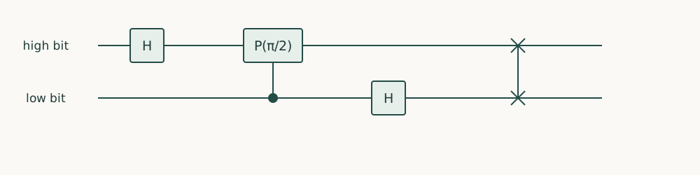
The circuit follows. H on qubit 1 makes \((\ket0+(-1)^{y_1}\ket1)/\sqrt2\). The controlled phase from qubit 0 must come next, while qubit 0 still holds the bit \(y_0\), and it completes the \(x_0\) factor, on qubit 1. H on qubit 0 then makes the \(x_1\) factor, on qubit 0. Each factor has ended up on the other wire, so a final swap puts them in place:
The companion compares all 16 entries of this circuit’s matrix with \(e^{2\pi ixy/4}/2\). The expected matrix is built by a list comprehension with two for clauses, one per index, and 2j is Python’s notation for the complex number \(2i\). Omitting the swap would reverse the output bit order. Taking the inverse would flip the sign of the exponent.
Positive-sign two-qubit Fourier circuit. The final SWAP exchanges the two wires; its connected endpoints are a two-wire operation. The controlled phase applies only when both bits are one.
Problem 8.1. Why compare QFT matrices instead of only transforming zero?
Worked solution
Both forward and inverse Fourier transforms map zero to the same uniform state. A zero-input test misses the sign convention.
8.1.2 Controlled powers and phase estimation
Phase estimation asks: given a unitary \(U\) and an eigenstate with \(U\ket u=e^{2\pi i\varphi}\ket u\), what is \(\varphi\)? We need a test case whose answer we know exactly. We choose \(U=P(2\pi\varphi)\) with \(\varphi=1/4\) and eigenstate \(\ket1\), prepared on qubit 2 with an X gate. Qubits 0 and 1 form the counting register.
We put each counting qubit in \(\ket+\) and let counting qubit \(j\) control \(U^{2^j}\). By phase kickback, qubit \(j\) picks up the phase \(e^{2\pi i\varphi2^j}\) on its \(\ket1\). Together the two qubits hold \[\frac12\sum_{x=0}^{3}e^{2\pi i\varphi x}\ket x.\] With \(\varphi=y/4\), this is exactly \(F\ket y\). So the inverse Fourier circuit returns \(\ket y\), here \(y=4\varphi=1\).
In the program, qft.inverse() supplies the inverse, and compose(…, qubits=[0, 1], inplace=True) attaches it to the counting wires, changing qpe itself rather than returning a copy. Here \(U^{2^j}\) is again a phase gate, so each power costs one controlled phase. For a general \(U\), implementing \(U^{2^j}\) by repetition costs \(2^j\) uses of \(U\).
The check asks for the probabilities of the counting qubits alone, probabilities([0, 1]), and requires that integer 1 has probability 1. We decode the counting register through this list of qubits, not through the order of wires in a drawing. A phase that is exactly representable in two bits makes the first test clean. Approximate phases and superpositions of eigenstates come after it passes.
8.2 Amplitude Manipulation
Phase estimation reads out a phase. Search uses phases differently: a phase oracle marks the good items with a sign, and reflections turn that sign into probability. The algorithm fixes the reflections only up to conventions. Which conventions are safe to choose freely, and how many iterations should the program run? We implement the reflections first, then the search loop.
8.2.1 Preparation and reflections
Take four items, with only \(\ket{11}\) marked. We begin with the uniform state \(\ket s=H^{\otimes2}\ket{00}\). How do we mark \(\ket{11}\) with a sign? A CZ gate multiplies exactly \(\ket{11}\) by \(-1\), so it is the phase oracle here.
Next comes the reflection about \(\ket s\), usually written \(D=2\ketbra ss-I\). The companion builds it as H on both, X on both, CZ, X on both, H on both. What does that sequence compute? Conjugating CZ by X on both qubits moves its sign from \(\ket{11}\) to \(\ket{00}\), giving \(I-2\ketbra{00}{00}\). Conjugating by H on both then gives \(I-2\ketbra ss=-D\).
So the companion implements \(-D\), which differs from the textbook reflection by a global sign. For the search alone that sign changes no probability. If the whole iteration were later controlled, though, it would become a relative phase on the control, by the result we derived for controlled operations. So the convention must be recorded with the component.
8.2.2 Search and amplification
How many iterations should we run? One marked item out of four gives initial success probability \(\sin^2\theta=1/4\), so \(\theta=\pi/6\). Each iteration rotates the state by \(2\theta\) toward the marked item, so after \(k\) iterations the success probability is \(\sin^2((2k+1)\theta)\). One iteration gives \(\sin^2(\pi/2)=1\). The companion checks that the probability of index 3, the state \(\ket{11}\), is 1.
Python allows several statements on one line when they are separated by semicolons, which keeps the reflection on two lines. For larger instances, we choose the number of iterations from the initial success probability. When that probability is unknown, we need a schedule with a justified guarantee. More iterations can reduce success, so a loop that simply runs “long enough” is not an algorithm.
Problem 8.2. What happens after a second Grover iteration in the four-item example?
Worked solution
The success returns to one quarter. The rotation has passed the good direction.
8.3 Quantum Walks
A quantum walk moves amplitude around a graph, one step at a time, steered by an extra register called the coin. To program it, we must make the step reversible with the gates we have, and then decide what a fair comparison with a classical walk would measure. We first implement one step on a four-site cycle, then ask what its cost and its correctness tests do and do not tell us.
8.3.1 Position and coin registers
Suppose a walker sits on a cycle of four sites. A step should move it one site forward or one site back. Can we write that step as a unitary on the position alone? No. Both “site 1 moved forward” and “site 3 moved back” end at site 2, so a position-only map would merge two states into one, and a unitary cannot do that. We add a coin qubit that records the direction. The step is then reversible, because the coin tells us which way to undo it.
We put the coin on qubit 0 and the position, \(q_1+2q_2\), on qubits 1 and 2. One step applies H to the coin and then shifts: coin 0 moves the position by \(+1\), coin 1 by \(-1\), both modulo 4. The increment is the two-bit incrementer we built for arithmetic oracles, with an extra control on the coin. The decrement is its inverse. To condition on coin 0 instead of coin 1, we surround the controlled increment with X gates on the coin:
walk = QuantumCircuit(3)
walk.h(0)
walk.cx(0, 1); walk.ccx(0, 1, 2) # coin 1: position - 1
walk.x(0); walk.ccx(0, 1, 2); walk.cx(0, 1); walk.x(0) # coin 0: position + 1
Our independent prediction is a matrix. The shift sends basis index \(c+2p\) to \(c+2((p\pm1)\bmod4)\), and the coin step is \(I\otimes H\), with H on the right because the coin is qubit 0. The companion builds both with NumPy: % is the remainder, so -1 % 4 is 3, and np.kron forms a tensor product. It then compares the circuit’s matrix with their product.
Two further rules follow from the reasoning above. We keep the coin from step to step, since discarding its direction after a step would turn the walk into a different, non-unitary process. And if the number of sites is not a power of two, some basis states of the position register stand for no site, so the circuit needs a stated rule for them to remain unitary.
Problem 8.3. Can the position register alone generally implement a reversible coined shift?
Worked solution
The direction label is needed to distinguish the routes. Removing it without another reversible encoding can merge states and invalidate the proposed unitary.
8.3.2 Implementation and classical baselines
Our walk passes its matrix check. Does that tell us anything about whether a quantum walk beats a classical one? No. A matrix check establishes correctness for one small instance. A fair comparison with a classical method must give both the same access to the graph and ask both for the same output. The quantum side should then be measured by quantities that grow with the instance: compiled gates, depth, qubits, oracle calls and readout cost.
What about the time our simulation took? That measures the classical simulator, not the quantum algorithm. A simulation that slows down rapidly with size says nothing about how the circuit would perform on quantum hardware. The companion collects the checks from this chapter: the Fourier matrix, the phase-estimation readout, the search success and the walk step. They establish correctness, not a performance advantage.
"""Runnable companion for Quantum Programming, Chapter 8."""
import numpy as np
from qiskit import QuantumCircuit
from qiskit.quantum_info import Operator, Statevector
# Positive-sign QFT on integer labels |q1 q0>.
qft = QuantumCircuit(2)
qft.h(1)
qft.cp(np.pi / 2, 0, 1)
qft.h(0)
qft.swap(0, 1)
expected = np.array([[np.exp(2j*np.pi*x*y/4)/2 for x in range(4)] for y in range(4)])
assert np.allclose(Operator(qft).data, expected)
# Phase estimation: counting qubits 0 and 1, eigenstate |1> of P(2*pi*phi) on qubit 2.
phi = 1 / 4
qpe = QuantumCircuit(3)
qpe.x(2)
qpe.h([0, 1])
for j in range(2):
    qpe.cp(2 * np.pi * phi * 2**j, j, 2)  # controlled U^(2^j)
qpe.compose(qft.inverse(), qubits=[0, 1], inplace=True)
counting = Statevector.from_instruction(qpe).probabilities([0, 1])
assert np.isclose(counting[1], 1) # integer 1 = phi * 4
# One Grover step for marked state |11> in four items.
search = QuantumCircuit(2)
search.h([0, 1])
search.cz(0, 1)
search.h([0, 1]); search.x([0, 1]); search.cz(0, 1)
search.x([0, 1]); search.h([0, 1])
assert np.isclose(Statevector.from_instruction(search).probabilities()[3], 1)
# One coined-walk step on a 4-cycle: coin q0, position q1 + 2*q2.
walk = QuantumCircuit(3)
walk.h(0)
walk.cx(0, 1); walk.ccx(0, 1, 2)                 # coin 1: position - 1
walk.x(0); walk.ccx(0, 1, 2); walk.cx(0, 1); walk.x(0)  # coin 0: position + 1
shift = np.zeros((8, 8))
for coin in range(2):
for position in range(4):
moved = (position + (1 if coin == 0 else -1)) % 4
shift[coin + 2 * moved, coin + 2 * position] = 1
coin_flip = np.kron(np.eye(4), np.array([[1, 1], [1, -1]]) / np.sqrt(2))
assert np.allclose(Operator(walk).data, shift @ coin_flip)
print(qft.draw(output="text"))
Each check in this chapter compared a program with a prediction we derived first. Some checks were stronger than others: a full matrix catches more than one probability. What, in general, counts as enough evidence that a quantum program does what it should?
Implementing Fourier, amplitude-amplification, and quantum-walk algorithms in code requires matching bit-reversal conventions, reflection phases, and oracle workspace uncomputation.
Small-scale statevector assertions verify that intermediate reflections and inverse QFT layers produce the exact theoretical amplitudes before adding shot noise.
Resource scaling should be measured empirically by sweeping register size \(n\) and recording transpiled two-qubit gate counts and circuit depth.
Questions and worked problems
These exercises draw on the whole chapter. Attempt each question before opening a hint, explain your reasoning, then compare it with the worked solution.
Verify that the inverse of the chapter’s positive-sign QFT matches \(e^{-2\pi ixy/4}/2\). Why is the sign convention worth an explicit test?
Hint 1
Build the expected matrix with the negative exponent.
Hint 2
Phase estimation uses the inverse transform.
Worked solution
qft.inverse() matches the matrix with \(e^{-2\pi ixy/4}/2\). Libraries and papers differ on which sign is “the” QFT, and phase estimation needs the inverse of whichever transform produced its phase ramp. A wrong sign returns \(-\phi\) (mod \(1\)) instead of \(\phi\), an error that a test on \(\ket0\) alone would miss, because both transforms send \(\ket0\) to the uniform state.
import numpy as np
from qiskit import QuantumCircuit
from qiskit.quantum_info import Operator

qft = QuantumCircuit(2)
qft.h(1)
qft.cp(np.pi / 2, 0, 1)
qft.h(0)
qft.swap(0, 1)
inverse = np.array([[np.exp(-2j * np.pi * x * y / 4) / 2 for x in range(4)] for y in range(4)])
assert np.allclose(Operator(qft.inverse()).data, inverse)
Modify the chapter’s four-item search to mark \(01\) (qubit 0 equal to \(1\), qubit 1 equal to \(0\)) instead of \(11\). Which gates change, and what probability does the marked index reach after one iteration?
Hint 1
X gates turn the marked pattern into \(11\) for the CZ.
Hint 2
Wrap the oracle’s CZ with X on qubit 1.
Worked solution
Only the oracle changes: apply X to qubit 1, then CZ, then X to qubit 1, so the sign falls on \(\ket{01}\). The diffusion step is unchanged. After one iteration, index \(1\) has probability \(1\). Separating the oracle from the diffusion makes this change local and testable.
Remove the final swap from the two-qubit QFT. Show that the result equals the full QFT followed by an extra swap. Is the swap-free circuit wrong?
Hint 1
SWAP is its own inverse.
Hint 2
Compare operators of ns + swap with qft.
Worked solution
The swap-free circuit followed by a swap equals the full QFT, so the swap-free version computes the same transform with its output qubits in reversed order. It is not wrong if the reversal is accounted for, for example by relabeling outputs or by absorbing it into later wiring; many implementations omit the swaps to save gates. It is wrong only if downstream code assumes the standard order.
Implement two-bit phase estimation for \(U=P(\pi/2)\), whose eigenstate \(\ket1\) has phase \(\phi=1/4\). Controls are qubits 0 (power \(1\)) and 1 (power \(2\)); the target is qubit 2 in \(\ket1\). Apply the controlled powers as controlled phases and then the inverse of the chapter’s QFT on the controls. Predict and verify the control readout.
Hint 1
\(U^2=P(\pi)\).
Hint 2
The control register ends in \(\ket j\) with \(j=4\phi=1\).
Worked solution
Controlled-\(U\) is cp(\(\pi/2\)) from qubit 0 and controlled-\(U^2\) is cp(\(\pi\)) from qubit 1. They write \(e^{2\pi ik/4}\) onto control basis state \(\ket k\), and the inverse QFT returns \(\ket{j}\) with \(j=1\). The full label is 101 (target 1, controls 01), with probability \(1\), so \(\phi=j/4=1/4\). Testing with an exactly representable phase first isolates convention errors from rounding effects.
Repeat phase estimation with three control qubits for a phase that is not exactly representable, \(\phi=1/3\). (a) Which outcome is most likely, and with what probability? (b) What estimate of \(\phi\) does it give? (c) How would you test this case, given that the outcome is random?
Hint 1
\(8\phi\approx2.67\), so expect \(j=3\) most often.
Hint 2
Compare the distribution with \(|a_j|^2=\sin^2(\pi M\Delta)/(M^2\sin^2\pi\Delta)\).
Worked solution
(a) The control readout \(j=3\) has probability about \(0.69\), with \(j=2\) next at about \(0.17\). (b) \(j=3\) gives \(\phi\approx3/8=0.375\), the nearest grid value to \(1/3\). (c) Compare the exact output distribution from Statevector with the analytic formula for every \(j\), rather than asserting a single outcome; in sampled runs, test that the frequency of \(j=3\) lies within a tolerance of \(0.69\).
import numpy as np
from qiskit import QuantumCircuit
from qiskit.quantum_info import Statevector

def inverse_qft(n):
    circuit = QuantumCircuit(n)
    for j in range(n // 2):
        circuit.swap(j, n - 1 - j)
    for j in range(n):
        for k in range(j):
            circuit.cp(-np.pi / 2 ** (j - k), k, j)
        circuit.h(j)
    return circuit

phi, m = 1 / 3, 3
circuit = QuantumCircuit(m + 1)
circuit.x(m)
circuit.h(range(m))
for j in range(m):
    circuit.cp(2 * np.pi * phi * 2 ** j, j, m)
circuit.compose(inverse_qft(m), qubits=range(m), inplace=True)
probabilities = Statevector.from_instruction(circuit).probabilities_dict(qargs=list(range(m)))
M = 2 ** m
for j in range(M):
    delta = phi - j / M
    analytic = np.sin(np.pi * M * delta) ** 2 / (M ** 2 * np.sin(np.pi * delta) ** 2)
    assert np.isclose(probabilities.get(format(j, "03b"), 0), analytic)
assert max(probabilities, key=probabilities.get) == "011"
Implement a coined walk on a four-cycle: qubit 0 is the coin, qubits 1 and 2 hold the position (low bit on qubit 1). Each step applies H to the coin, increments the position if the coin is \(1\), and decrements it if the coin is \(0\). Starting from coin \(0\) at position \(0\), predict the position distribution after three steps and verify it.
Hint 1
A controlled two-bit incrementer is ccx(coin, p0, p1) followed by cx(coin, p0).
Hint 2
Decrement is the inverse of increment, controlled on coin \(0\) (wrap the controls with X).
Worked solution
After three steps the walker is at position \(3\) with certainty: interference cancels every route to position \(1\). The controlled increment is ccx(0, 1, 2), cx(0, 1); the decrement controlled on coin \(0\) is X on the coin, then cx(0, 1), ccx(0, 1, 2), then X on the coin. A classical random walk would be at position \(1\) or \(3\) with probability \(\frac12\) each; the coin register must be kept, not measured, for the interference to occur.
import numpy as np
from qiskit import QuantumCircuit
from qiskit.quantum_info import Statevector

def step(circuit):
    circuit.h(0)
    circuit.ccx(0, 1, 2)   # increment when coin is 1
    circuit.cx(0, 1)
    circuit.x(0)           # decrement when coin is 0
    circuit.cx(0, 1)
    circuit.ccx(0, 1, 2)
    circuit.x(0)

walk = QuantumCircuit(3)
for _ in range(3):
    step(walk)
positions = Statevector.from_instruction(walk).probabilities_dict(qargs=[1, 2])
assert np.isclose(positions["11"], 1)
Implement Grover search for one marked item, \(111\), among eight. Use H, Toffoli, H on qubit 2 as the controlled-controlled-Z oracle, and the standard diffusion. Compute the success probability after \(0,1,2,3\) iterations and compare with \(\sin^2((2k+1)\theta)\), \(\sin\theta=1/\sqrt8\).
Hint 1
The best number of iterations is \(2\).
Hint 2
Diffusion: H on all, X on all, controlled-controlled-Z, X on all, H on all.
Worked solution
The success probabilities are \(0.125\), \(0.781\), \(0.945\), and \(0.330\) for \(k=0,1,2,3\), exactly \(\sin^2((2k+1)\theta)\). The third iteration overshoots. The test compares each value with the formula, which checks both the oracle and the diffusion, and documents why the iteration count is a parameter derived from \(N\), not a loop that runs until some budget is exhausted.
import numpy as np
from qiskit import QuantumCircuit
from qiskit.quantum_info import Statevector

def ccz(circuit):
    circuit.h(2)
    circuit.ccx(0, 1, 2)
    circuit.h(2)

def grover(iterations):
    circuit = QuantumCircuit(3)
    circuit.h([0, 1, 2])
    for _ in range(iterations):
        ccz(circuit)
        circuit.h([0, 1, 2]); circuit.x([0, 1, 2])
        ccz(circuit)
        circuit.x([0, 1, 2]); circuit.h([0, 1, 2])
    return Statevector.from_instruction(circuit).probabilities()[7]

theta = np.arcsin(1 / np.sqrt(8))
for k in range(4):
    assert np.isclose(grover(k), np.sin((2 * k + 1) * theta) ** 2)
A student tests a QFT implementation only on the input \(\ket{00}\), checks that the output is the uniform superposition, and declares it correct. Construct a wrong circuit that passes this test, and state a test that would catch it.
Hint 1
Any circuit that applies H to each qubit sends \(\ket{00}\) to the uniform state.
Hint 2
Compare full operators, or test several inputs with phases.
Worked solution
\(H\otimes H\) alone sends \(\ket{00}\) to the uniform superposition, exactly like the QFT, and so does the inverse QFT. All three differ on other inputs; for example the QFT and \(H\otimes H\) give different phases on \(\ket{01}\). A correct test compares the full operator with the defining matrix (as the chapter does), or checks every basis input including relative phases. A single input exercises only one column of the matrix.
import numpy as np
from qiskit import QuantumCircuit
from qiskit.quantum_info import Operator, Statevector

hh = QuantumCircuit(2)
hh.h([0, 1])
assert Statevector.from_instruction(hh).equiv(Statevector([0.5, 0.5, 0.5, 0.5]))
qft_matrix = np.array([[np.exp(2j * np.pi * x * y / 4) / 2 for x in range(4)] for y in range(4)])
assert not np.allclose(Operator(hh).data, qft_matrix)
Build a four-qubit positive-sign QFT and an approximate version that omits the smallest controlled phase, cp(\(\pi/8\)). (a) Compute the operator-norm distance between them. (b) Compare it with the bound \(|e^{i\pi/8}-1|\). (c) How does this scale to large registers?
Hint 1
A controlled phase differs from the identity by \(e^{i\theta}-1\) on one basis state.
Hint 2
Use numpy’s matrix 2-norm of the difference.
Worked solution
(a) The distance is about \(0.390\). (b) That equals \(|e^{i\pi/8}-1|\approx0.390\): removing one controlled phase changes the circuit by exactly that gate’s deviation from the identity, because unitaries before and after it preserve norms. (c) Dropping every rotation smaller than \(2\pi/2^b\) gives total error below about \(2\pi n/2^b\) with only \(O(n\log n)\) gates, the approximate QFT of Quantum Algorithms; omitting larger angles, as here, gives a large error.
import numpy as np
from qiskit import QuantumCircuit
from qiskit.quantum_info import Operator

def inverse_qft(n):
    circuit = QuantumCircuit(n)
    for j in range(n // 2):
        circuit.swap(j, n - 1 - j)
    for j in range(n):
        for k in range(j):
            circuit.cp(-np.pi / 2 ** (j - k), k, j)
        circuit.h(j)
    return circuit

exact = inverse_qft(4).inverse()
approximate = QuantumCircuit(4)
for instruction in exact.data:
    if instruction.operation.name == "cp" and np.isclose(abs(float(instruction.operation.params[0])), np.pi / 8):
        continue
    approximate.append(instruction)
distance = np.linalg.norm(Operator(exact).data - Operator(approximate).data, 2)
assert np.isclose(distance, abs(np.exp(1j * np.pi / 8) - 1))
In phase estimation with \(m\) control qubits, controlled-\(U^{2^j}\) built by repetition needs \(2^j\) uses of controlled-\(U\). (a) Count the total uses for \(m=3\) and \(m=10\). (b) For \(U=P(\lambda)\), what shortcut implements \(U^{2^j}\) at the cost of one gate? (c) Why does a benchmark of phase estimation need to state which of these was used?
Hint 1
Total \(2^m-1\).
Hint 2
\(P(\lambda)^k=P(k\lambda)\).
Worked solution
(a) \(m=3\): \(7\) uses; \(m=10\): \(1023\). (b) \(P(\lambda)^{2^j}=P(2^j\lambda)\), a single controlled phase, which is why the worked problems used cp(\(2^j\lambda\)) directly. (c) With repetition, the circuit grows exponentially in the number of bits of precision; with a shortcut, linearly. Modular multiplication in Shor’s algorithm has such a shortcut, while general Hamiltonian evolution does not. A runtime or gate count is meaningless without saying which construction was used.