Education / Quantum Information

Quantum Information · Chapter 07

Quantum Measurement

What can a measuring procedure reveal, and what does it leave behind?

In this chapter
  1. 7.1 Measurement Procedures
    1. 7.1.1 Coupling to an auxiliary system
    2. 7.1.2 Outcomes and conditional operations
  2. 7.2 General Measurements
    1. 7.2.1 Measurement effects and probabilities
    2. 7.2.2 POVMs and physical implementations
  3. 7.3 Information and Disturbance
    1. 7.3.1 Outcome statistics versus state updates
    2. 7.3.2 Sequential measurement and retained records
Before you begin

Starting point: Projective measurement and channels built from ancillas; measurement effects and state updates are derived from circuits.

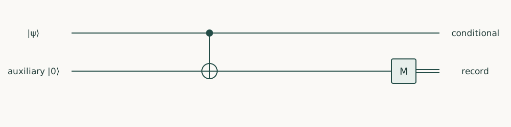
Keep in view: An ancilla-assisted measurement of a qubit.

Any physical process on a qubit can be built from an ancilla, a joint unitary and a discarded output. On the qubit alone it acts as a channel, a few Kraus operators sandwiching the density operator. We also saw that reading the ancilla, instead of discarding it, turns a CNOT record into a Z measurement.

That observation raises two questions. Our only measurements so far are projective, yet a real detector can be noisy, and a noisy detector is no projector. And two detectors with the same outcome frequencies may leave the system in different states. What describes a measurement in general? Reading an ancilla gives one operator per outcome, which fixes both the probability and the state left behind. Asking which part the probabilities actually use leaves a smaller object, the effect. The effects of a measurement form a POVM, and every POVM can be built from an ancilla. The full set of state changes is a larger object, the instrument, and sequential measurements show why it is needed.

7.1 Measurement Procedures

A detector couples to a system and then shows a result. What does that result tell us, and what state does it leave? We describe the general procedure by sorting the joint state by the ancilla's label, as we did for channels, and then reading the label. The CNOT record checks that this reproduces the projective measurement we already know, for pure and mixed inputs alike.

7.1.1 Coupling to an auxiliary system§

A system in \(\ket\psi\) meets an ancilla in \(\ket0\), and a joint unitary \(U\) acts. Then we read the ancilla in its computational basis. Which outcome do we see, and what is the system's state afterwards?

Sort the joint output by the ancilla's label, exactly as for a channel:

\[U\ket\psi\ket0=\sum_j\bigl(M_j\ket\psi\bigr)\ket j,\qquad M_j=\bra jU\ket0.\]

Reading the ancilla is a projective measurement on it. The projector for outcome \(j\) keeps the term \((M_j\ket\psi)\ket j\), so outcome \(j\) has probability \(p_j=\|M_j\ket\psi\|^2\). Given that outcome, the system is left in \(M_j\ket\psi/\sqrt{p_j}\).

For a mixed input we average over an ensemble, as before. The unnormalized branch is \(M_j\rho M_j^\dagger\). Its trace is the probability, and dividing by it gives the conditional state:

\[p_j=\mathrm{tr}\bigl(M_j\rho M_j^\dagger\bigr),\qquad\rho_j=\frac{M_j\rho M_j^\dagger}{p_j}\quad(p_j>0).\]

The \(M_j\) are the measurement operators of the procedure. They are the Kraus operators of the channel we would get by discarding the ancilla. The only difference is that we now keep the record.

7.1.2 Outcomes and conditional operations§

Does the general rule agree with the measurement postulate when it should? Take the CNOT record. Its measurement operators are \(M_0=\ket0\bra0\) and \(M_1=\ket1\bra1\), the projectors of the Z measurement. So reading the ancilla carries out a Z measurement of the system, with the probabilities and updates of the postulate.

Measure the auxiliary after CNOT to record the system’s Z value. Ignoring the record gives dephasing; conditioning on it gives a projective state update.

Follow a plus input. CNOT produces a Bell pair. Reading the ancilla gives 0 or 1, each with probability \(1/2\). On the 0 branch the system is \(\ket0\), and on the 1 branch it is \(\ket1\). What we should predict next depends on what we keep. If we keep the label, we use the branch state. If we ignore the label, we average the branches and get \(I/2\).

The mixed-input rule behaves the same way. Dividing \(M_j\rho M_j^\dagger\) by its trace is the density-operator version of dividing a projected vector by its length. A branch with zero probability has no conditional state, because nothing is left to normalize.

Problems

Problem 7.1. On plus input, compare conditioning on auxiliary outcome zero with ignoring the auxiliary record.

Worked solution

Conditioning selects the zero branch, with probability one half, leaving the system in zero. Ignoring the record averages both branches and leaves I/2. The normalized conditional state and the unconditioned state answer different prediction questions.

7.2 General Measurements

An ancilla reproduced the Z measurement, but most ancilla constructions give operators that are not projectors. Which object predicts the outcome probabilities of such a measurement? We start from a detector that sometimes misreports, which no projective measurement describes. Its probabilities lead to effects, and the ancilla picture shows that effects are all the probabilities use. Then we reverse the question and build a device for any valid set of effects.

7.2.1 Measurement effects and probabilities§

A Z detector misreports its result one time in four. It might, for instance, measure Z perfectly and then flip the displayed result on a quarter of the trials. On input \(\rho\) it reports 0 with probability \(\tfrac34\rho_{00}+\tfrac14\rho_{11}\). Is this a projective measurement in some basis?

The probability is linear in \(\rho\), so we can write it with a matrix. Let \(E_0=\mathrm{diag}(3/4,1/4)\), where diag lists the diagonal entries of a matrix that is zero elsewhere:

\[p_0=\mathrm{tr}(E_0\rho),\qquad p_1=\mathrm{tr}(E_1\rho),\qquad E_1=I-E_0.\]

The probabilities for all inputs fix \(E_0\): the inputs \(\ket0\) and \(\ket1\) give its diagonal entries, and inputs such as \(\ket+\) give the rest. A projector \(P\) satisfies \(P^2=P\), because keeping a component twice is the same as keeping it once. But \(E_0^2=\mathrm{diag}(9/16,1/16)\neq E_0\). So no projective measurement, in any basis, has these statistics.

How does such a matrix arise from measurement operators? Moving \(M_j^\dagger\) around the trace, as we did for channels, gives \(p_j=\mathrm{tr}(M_j\rho M_j^\dagger)=\mathrm{tr}(M_j^\dagger M_j\rho)\). So the probabilities use only

\[E_j=M_j^\dagger M_j.\]

This matrix is the effect of outcome \(j\). Different measurement operators can share an effect. Replacing \(M_j\) by \(VM_j\) for any unitary \(V\) leaves \(E_j\) unchanged, because \(V^\dagger V=I\).

Which matrices can be effects? Each probability is nonnegative, and \(\bra v E_j\ket v=\|M_j\ket v\|^2\geq0\), so every effect is positive. The probabilities add to one for every input. The ancilla construction guarantees this, since \(\sum_jM_j^\dagger M_j=\bra0U^\dagger U\ket0=I\). A list of positive matrices adding to \(I\) is called a positive-operator-valued measure, or POVM.

A projective measurement is the special case in which every effect is a projector. A projector has eigenvalues 0 and 1 only. The eigenvalues of an effect can lie anywhere from 0 to 1, like the \(3/4\) and \(1/4\) of our detector.

7.2.2 POVMs and physical implementations§

Every ancilla construction gives a POVM. Can every POVM be built from an ancilla? Try the noisy detector. The flip-the-display version measures Z fully and leaves \(\ket0\) or \(\ket1\). We look for a device with the same effects that disturbs the qubit less.

First we need measurement operators with \(M_j^\dagger M_j=E_j\). For this diagonal effect we can take square roots of the diagonal entries: \(M_0=\mathrm{diag}(\sqrt3/2,1/2)\) and \(M_1=\mathrm{diag}(1/2,\sqrt3/2)\). Next we need a unitary that produces \(\sum_j(M_j\ket\psi)\ket j\). Look at what it must do to each system label:

\[\ket0\ket0\mapsto\ket0\bigl(\tfrac{\sqrt3}2\ket0+\tfrac12\ket1\bigr),\qquad\ket1\ket0\mapsto\ket1\bigl(\tfrac12\ket0+\tfrac{\sqrt3}2\ket1\bigr).\]

This is a controlled rotation. If the system is 0, the ancilla is turned by the angle \(\pi/6\), and if it is 1, by \(\pi/3\), where a turn by \(\theta\) is the real unitary \(\bigl(\begin{smallmatrix}\cos\theta&-\sin\theta\\\sin\theta&\cos\theta\end{smallmatrix}\bigr)\). Each rotation is unitary, so the whole operation is unitary. Reading the ancilla then gives exactly \(M_0\) and \(M_1\).

The general case follows the same plan. For any POVM choose \(M_j\) with \(M_j^\dagger M_j=E_j\). The map \(\ket\psi\mapsto\sum_j(M_j\ket\psi)\ket j\) keeps inner products, because \(\sum_j\bra\phi M_j^\dagger M_j\ket\psi=\braket\phi\psi\). It is defined only on inputs with the ancilla in \(\ket0\). Extending it to a unitary on all inputs means completing a set of orthonormal columns, which is always possible; we take that standard linear-algebra fact as given. So every POVM can be realized physically.

What does the noisy detector do to plus? Outcome 0 has probability \(\tfrac34\cdot\tfrac12+\tfrac14\cdot\tfrac12=\tfrac12\). The unnormalized branch is \(M_0\ket+=(\sqrt3\ket0+\ket1)/(2\sqrt2)\), with squared length \(1/2\). Normalizing gives \((\sqrt3\ket0+\ket1)/2\). The detector has nudged the state towards \(\ket0\) without projecting onto it.

Problems

Problem 7.2. Verify the square-root implementation’s completeness.

Worked solution

M0†M0+M1†M1=E0+E1=I, so total outcome probability is one for every input.

7.3 Information and Disturbance

A POVM fixes every outcome probability. Does it also fix what the measurement does to the system? We show that it does not, by changing the state after each outcome while leaving the effects alone. A second measurement then exposes the difference, and the noisy detector shows that even a weakly informative measurement leaves an observable disturbance.

7.3.1 Outcome statistics versus state updates§

Suppose that after outcome \(j\) the device applies a unitary \(V_j\) of its own. The measurement operator becomes \(V_jM_j\), but the effect \((V_jM_j)^\dagger V_jM_j=M_j^\dagger M_j\) is unchanged. Every outcome probability is the same. Is the measurement the same?

Compare two Z detectors. The first is the ordinary one: after outcome \(j\) it leaves \(\ket j\). The second applies \(X\) after outcome 1, so it always leaves \(\ket0\). Its measurement operators are \(\ket0\bra0\) and \(\ket0\bra1\). On any input the two detectors report 0 and 1 with identical probabilities. Yet one leaves the observed state and the other resets the qubit.

So outcome probabilities do not determine the state change. The full list of branch maps \(\rho\mapsto M_j\rho M_j^\dagger\), one for each outcome, is called an instrument. A POVM is what the instrument tells us about probabilities alone.

7.3.2 Sequential measurement and retained records§

How could anyone tell the two Z detectors apart? Measure twice. On input \(\ket1\), the ordinary detector followed by another Z measurement reports 1 and then 1. The resetting detector reports 1 and then 0. The second measurement sees what the first left behind.

Does a weakly informative measurement escape disturbance? Return to the noisy detector on plus, and ignore its outcome. Each branch contributes an off-diagonal entry \(\sqrt3/8\), so the averaged output is

\[\frac12\begin{pmatrix}1&\sqrt3/2\\\sqrt3/2&1\end{pmatrix}.\]

A later plus test succeeds with probability \((1+\sqrt3/2)/2\approx0.933\), instead of 1. The detector revealed only a little about the Z value, and it disturbed the state only a little, but the disturbance is observable.

The instrument matters here too. Append \(Z\) to every branch. The first outcome statistics are identical, but the off-diagonal entries reverse sign, and the plus test now succeeds with probability \((1-\sqrt3/2)/2\approx0.067\). Recording an outcome, ignoring it, and acting on it are different operations, and each must be stated.

We can now describe any measurement, its probabilities and its aftermath. Suppose Bob knows that Alice sent one of two known states. Which measurement should he choose, and how often can he be right?

Problems

Problem 7.3. Why is a POVM insufficient to predict sequential measurements?

Worked solution

It specifies each first outcome probability, but not the conditional output state. The next measurement depends on the instrument, including any outcome-dependent transformations.

Transfer problem. For the noisy square-root measurement and plus input, predict the probability of two consecutive zero records, using the same instrument both times. Are the two records independent?

Worked solution

The first zero has probability 1/2 and leaves \((\sqrt3\ket0+\ket1)/2\). The next zero probability is \((3/4)(3/4)+(1/4)(1/4)=5/8\). The joint probability is 5/16, not 1/4. State disturbance correlates the two records.

Summary

Questions and worked problems

These exercises draw on the whole chapter. Attempt each question before opening a hint, explain your reasoning, then compare it with the worked solution.

1. Quick check §

Which of these pairs is a valid two-outcome POVM? (a) \(E_0=\mathrm{diag}(0.9,0.2)\), \(E_1=\mathrm{diag}(0.1,0.8)\); (b) \(E_0=\mathrm{diag}(1.1,0.5)\), \(E_1=\mathrm{diag}(-0.1,0.5)\); (c) \(E_0=\ket+\bra+\), \(E_1=\ket-\bra-\). For the valid ones, give the outcome probabilities on \(\ket0\).

Hint 1

Check positivity of each effect and \(E_0+E_1=I\).

Hint 2

\(p_j=\bra0E_j\ket0\).

Worked solution

(a) Valid: both effects are positive and they sum to \(I\). On \(\ket0\), \(p_0=0.9\) and \(p_1=0.1\). (b) Invalid: \(E_1\) has a negative entry, which would give probability \(-0.1\) on \(\ket0\), even though the effects sum to \(I\). (c) Valid, and projective: on \(\ket0\) each outcome has probability \(\frac12\). Effect (a) is not a projector, since \(0.9^2\neq0.9\): it reports the \(Z\) value unreliably.

Revisit the relevant explanation

2. Quick check §

The noisy effect \(E_0=\mathrm{diag}(\frac34,\frac14)\), \(E_1=I-E_0\), is applied to \(\ket0\), \(\ket1\), and \(I/2\). Give \(p_0\) in each case. If \(\ket0\) and \(\ket1\) are equally likely a priori and the outcome is \(0\), what is the probability that the input was \(\ket0\)?

Hint 1

\(p_0=\mathrm{tr}(E_0\rho)\).

Hint 2

Use conditioning, as with the cards and the lamp.

Worked solution

\(p_0=\frac34\) for \(\ket0\), \(\frac14\) for \(\ket1\), and \(\frac12\) for \(I/2\). With equal priors, \(p(\ket0\mid0)=\frac{\frac12\cdot\frac34}{\frac12\cdot\frac34+\frac12\cdot\frac14}=\frac34\). The outcome is evidence about the \(Z\) value, like Bob’s lamp for the cards, rather than a sharp answer.

Revisit the relevant explanation

3. Quick check §

Let \(\ket{\psi_k}=\cos\frac{2\pi k}{3}\ket0+\sin\frac{2\pi k}{3}\ket1\) for \(k=0,1,2\), and \(E_k=\frac23\ket{\psi_k}\bra{\psi_k}\). Check that \(\sum_kE_k=I\) and compute the three outcome probabilities on \(\ket0\). Can a two-dimensional system have a three-outcome measurement?

Hint 1

The average of the projectors is \(\frac13\sum_k\ket{\psi_k}\bra{\psi_k}=I/2\).

Hint 2

\(\braket0{\psi_k}=\cos\frac{2\pi k}{3}\).

Worked solution

Since \(\frac13\sum_k\ket{\psi_k}\bra{\psi_k}=\frac I2\), we get \(\sum_kE_k=\frac23\cdot\frac32I=I\), and each effect is positive. On \(\ket0\), \(p_k=\frac23\cos^2\frac{2\pi k}{3}\): \(\frac23\), \(\frac16\), \(\frac16\). A qubit can have a measurement with more outcomes than its dimension; the effects are then not orthogonal projectors, and an ancilla is needed to realize it with a projective readout.

Revisit the relevant explanation

4. Worked problem §

Generalize the square-root measurement: \(E_0=\mathrm{diag}(q,1-q)\), \(M_j=\sqrt{E_j}\), applied to \(\ket+\). (a) Find the outcome probabilities and the conditional state after outcome \(0\). (b) If the outcome is ignored, show that the output coherence is \(\sqrt{q(1-q)}\) and find the probability that a later \(\pm\) test gives \(+\). (c) Evaluate at \(q=\frac12\), \(q=0.9\), and \(q=1\), and describe the trade-off.

Hint 1

\(M_0\ket+=(\sqrt q\ket0+\sqrt{1-q}\ket1)/\sqrt2\).

Hint 2

Each branch contributes off-diagonal \(\frac12\sqrt{q(1-q)}\).

Worked solution

(a) Each outcome has probability \(\frac12\); after outcome \(0\) the state is \(\sqrt q\ket0+\sqrt{1-q}\ket1\). (b) The branches contribute off-diagonal entries \(\frac12\sqrt{q(1-q)}\) each, totalling \(\sqrt{q(1-q)}\), so \(p(+)=\frac12+\sqrt{q(1-q)}\). (c) At \(q=\frac12\) the measurement learns nothing about \(Z\) and \(p(+)=1\): no disturbance. At \(q=0.9\), \(p(+)=0.8\). At \(q=1\), a sharp \(Z\) measurement, \(p(+)=\frac12\): full dephasing. The more the outcome reveals about \(Z\), the more coherence in the \(\pm\) basis it destroys, for this family of implementations.

Revisit the relevant explanation

5. Worked problem §

A system qubit controls a rotation of an ancilla in \(\ket0\): \(\ket0\ket0\mapsto\ket0\ket0\), \(\ket1\ket0\mapsto\ket1(\cos\frac\theta2\ket0+\sin\frac\theta2\ket1)\), and the ancilla is then measured. (a) Find \(M_0,M_1\) and the effects. (b) Which conclusion is certain when the outcome is \(1\)? (c) For input \(\ket+\), give the outcome probabilities and conditional states.

Hint 1

\(M_0=\mathrm{diag}(1,\cos\frac\theta2)\) and \(M_1=\mathrm{diag}(0,\sin\frac\theta2)\).

Hint 2

\(E_1=\mathrm{diag}(0,\sin^2\frac\theta2)\) vanishes on \(\ket0\).

Worked solution

(a) \(M_0=\mathrm{diag}(1,\cos\frac\theta2)\) and \(M_1=\mathrm{diag}(0,\sin\frac\theta2)\), with effects \(E_0=\mathrm{diag}(1,\cos^2\frac\theta2)\) and \(E_1=\mathrm{diag}(0,\sin^2\frac\theta2)\). (b) Outcome \(1\) never occurs for \(\ket0\), so it certifies that the input was not \(\ket0\), and leaves the system in \(\ket1\). (c) For \(\ket+\), \(p_1=\frac12\sin^2\frac\theta2\) and the state becomes \(\ket1\); \(p_0=\frac12(1+\cos^2\frac\theta2)\), leaving \((\ket0+\cos\frac\theta2\ket1)/\sqrt{1+\cos^2\frac\theta2}\). The outcome-\(0\) branch is still a superposition, tilted toward \(\ket0\): a one-sided, partial measurement.

Revisit the relevant explanation

6. Worked problem §

A qubit is known to be \(\ket0\) or \(\ket1\), each with prior probability \(\frac12\). The noisy instrument \(M_j=\sqrt{E_j}\) with \(E_0=\mathrm{diag}(\frac34,\frac14)\) is applied \(n\) times. (a) Why does the state stay \(\ket0\) or \(\ket1\) between rounds? (b) If \(k\) of the \(n\) records are \(0\), find the posterior odds for \(\ket0\). (c) How many records, with all zeros, give posterior probability above \(0.99\)?

Hint 1

\(M_j\) is diagonal, so it maps \(\ket0\) and \(\ket1\) to multiples of themselves.

Hint 2

Each record \(0\) multiplies the odds by \(3\), each record \(1\) by \(\frac13\).

Worked solution

(a) The branch operators are diagonal, so \(\ket0\) and \(\ket1\) are left unchanged up to normalization: repeated rounds give independent noisy readings of the same value. (b) A record \(0\) has likelihood ratio \(\frac{3/4}{1/4}=3\) in favor of \(\ket0\), and a record \(1\) has ratio \(\frac13\). The posterior odds are \(3^k\cdot3^{-(n-k)}=3^{2k-n}\). (c) With all zeros the odds are \(3^n\), and probability above \(0.99\) needs \(3^n>99\), so \(n=5\) (\(3^5=243\)). A weak measurement repeated on an undisturbed basis state accumulates into a sharp one.

Revisit the relevant explanation

7. Worked problem §

Use the trine measurement \(E_k=\frac23\ket{\psi_k}\bra{\psi_k}\) to identify which of the three trine states \(\ket{\psi_0},\ket{\psi_1},\ket{\psi_2}\) was prepared, each with probability \(\frac13\), guessing \(j\) on outcome \(j\). (a) Compute \(p(k\mid j)\). (b) Find the success probability. (c) Compare with guessing without measuring.

Hint 1

\(|\braket{\psi_k}{\psi_j}|^2=\cos^2(120^\circ)=\frac14\) for \(k\neq j\).

Hint 2

\(p(k\mid j)=\frac23|\braket{\psi_k}{\psi_j}|^2\).

Worked solution

(a) \(p(j\mid j)=\frac23\) and \(p(k\mid j)=\frac23\cdot\frac14=\frac16\) for \(k\neq j\); the three probabilities add to \(1\). (b) The success probability is \(\frac23\). (c) Guessing blindly succeeds with \(\frac13\). The three states are pairwise nonorthogonal, so no measurement identifies them perfectly, and a two-outcome projective measurement cannot even produce three different answers. The three-outcome POVM is the natural tool, and \(\frac23\) is known to be optimal for this ensemble.

Revisit the relevant explanation

8. Misconception §

A student says: “A weak measurement, one that barely distinguishes \(\ket0\) from \(\ket1\), causes negligible disturbance, so it can be repeated freely.” Using the square-root instrument with \(q=0.9\), whose ignored outcome multiplies the coherence by \(2\sqrt{q(1-q)}=0.6\), find the coherence of \(\ket+\) after \(10\) unrecorded rounds. What happens to a later \(\pm\) test?

Hint 1

Each round multiplies the off-diagonal entry by \(0.6\).

Hint 2

\(p(+)=\frac12+\rho_{01}\) for a real coherence.

Worked solution

Starting from coherence \(\frac12\), ten rounds give \(\frac12(0.6)^{10}\approx0.003\). A later \(\pm\) test gives \(+\) with probability about \(0.503\), essentially a fair coin, compared with certainty before any measurement. Each round disturbs the state only partly, but the disturbance accumulates multiplicatively. “Weak” describes the information gained per round, not a guarantee of small disturbance over a sequence; the total information gained about \(Z\) grows with the number of rounds, and so does the loss of \(\pm\) coherence.

Revisit the relevant explanation

9. Extension §

Construct an ancilla unitary that realizes the square-root instrument for \(E_0=\mathrm{diag}(\frac34,\frac14)\). (a) Define \(U\ket0\ket0=\ket0\big(\frac{\sqrt3}{2}\ket0+\frac12\ket1\big)\) and \(U\ket1\ket0=\ket1\big(\frac12\ket0+\frac{\sqrt3}{2}\ket1\big)\), and show that measuring the ancilla gives branch operators \(\sqrt{E_0}\) and \(\sqrt{E_1}\). (b) Check that \(U\) preserves the inner products of the two inputs. (c) Describe \(U\) as a pair of controlled rotations.

Hint 1

\(\bra0_E U\ket0_E=\mathrm{diag}(\frac{\sqrt3}{2},\frac12)\).

Hint 2

The two output states have different system labels, so they are orthogonal.

Worked solution

(a) Reading off the ancilla-\(0\) amplitudes gives \(M_0=\mathrm{diag}(\frac{\sqrt3}{2},\frac12)=\sqrt{E_0}\), and the ancilla-\(1\) amplitudes give \(M_1=\mathrm{diag}(\frac12,\frac{\sqrt3}{2})=\sqrt{E_1}\). (b) The two images have norm \(1\) and are orthogonal because their system labels differ, so the map preserves inner products on the subspace with ancilla \(\ket0\) and extends to a unitary on both qubits. (c) If the system is \(0\), rotate the ancilla so that it reads \(1\) with probability \(\frac14\); if the system is \(1\), rotate it so that it reads \(1\) with probability \(\frac34\). Every POVM can be realized this way: entangle with an ancilla, then measure the ancilla projectively.

Revisit the relevant explanation

10. Extension §

The same POVM \(E_0=\mathrm{diag}(\frac34,\frac14)\) can be implemented by measuring \(Z\) sharply and then reporting the opposite result with probability \(\frac14\). (a) Check that this produces the same outcome probabilities for every input. (b) For input \(\ket+\) with the outcome ignored, compare the output state with that of the square-root instrument, and compute the later \(\pm\) test probability for each. (c) What does this show about specifying a measurement?

Hint 1

The relabelled procedure has effects \(\frac34P_0+\frac14P_1\) and \(\frac14P_0+\frac34P_1\).

Hint 2

After a sharp \(Z\) measurement, every branch is diagonal.

Worked solution

(a) Outcome \(0\) occurs with probability \(\frac34\) on \(\ket0\) and \(\frac14\) on \(\ket1\), so the effect is \(\frac34P_0+\frac14P_1=E_0\): the same POVM. (b) The relabelled procedure collapses the state first, so with the outcome ignored the output is \(I/2\) and \(p(+)=\frac12\). The square-root instrument leaves coherence \(\frac{\sqrt3}{4}\), giving \(p(+)=\frac12+\frac{\sqrt3}{4}\approx0.933\). (c) Two devices with identical outcome statistics can disturb the system very differently. A POVM fixes the probabilities; predicting what happens next requires the full instrument, the set of branch maps.

Revisit the relevant explanation
Search this book

Search the course.